
Date: 2019-12-25 21:40:16 CET, cola version: 1.3.2
Document is loading...
All available functions which can be applied to this res_list object:
res_list
#> A 'ConsensusPartitionList' object with 24 methods.
#>   On a matrix with 51941 rows and 51 columns.
#>   Top rows are extracted by 'SD, CV, MAD, ATC' methods.
#>   Subgroups are detected by 'hclust, kmeans, skmeans, pam, mclust, NMF' method.
#>   Number of partitions are tried for k = 2, 3, 4, 5, 6.
#>   Performed in total 30000 partitions by row resampling.
#>
#> Following methods can be applied to this 'ConsensusPartitionList' object:
#>  [1] "cola_report"           "collect_classes"       "collect_plots"         "collect_stats"
#>  [5] "colnames"              "functional_enrichment" "get_anno_col"          "get_anno"
#>  [9] "get_classes"           "get_matrix"            "get_membership"        "get_stats"
#> [13] "is_best_k"             "is_stable_k"           "ncol"                  "nrow"
#> [17] "rownames"              "show"                  "suggest_best_k"        "test_to_known_factors"
#> [21] "top_rows_heatmap"      "top_rows_overlap"
#>
#> You can get result for a single method by, e.g. object["SD", "hclust"] or object["SD:hclust"]
#> or a subset of methods by object[c("SD", "CV")], c("hclust", "kmeans")]
The call of run_all_consensus_partition_methods() was:
#> run_all_consensus_partition_methods(data = mat, mc.cores = 4, anno = anno)
Dimension of the input matrix:
mat = get_matrix(res_list)
dim(mat)
#> [1] 51941 51
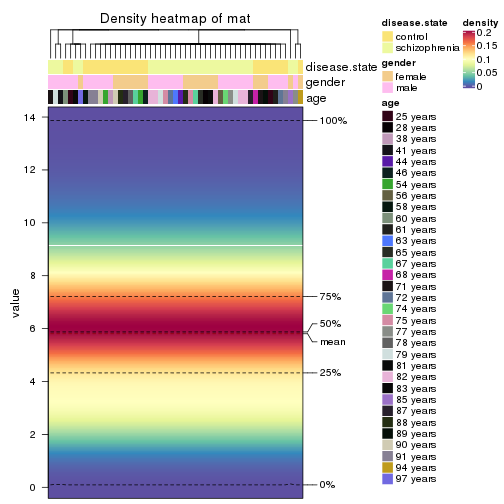
The density distribution for each sample is visualized as in one column in the following heatmap. The clustering is based on the distance which is the Kolmogorov-Smirnov statistic between two distributions.
library(ComplexHeatmap)
densityHeatmap(mat, top_annotation = HeatmapAnnotation(df = get_anno(res_list),
    col = get_anno_col(res_list)), ylab = "value", cluster_columns = TRUE, show_column_names = FALSE,
    mc.cores = 4)
Folowing table shows the best k (number of partitions) for each combination
of top-value methods and partition methods. Clicking on the method name in
the table goes to the section for a single combination of methods.
The cola vignette explains the definition of the metrics used for determining the best number of partitions.
suggest_best_k(res_list)
| The best k | 1-PAC | Mean silhouette | Concordance | Optional k | ||
|---|---|---|---|---|---|---|
| ATC:skmeans | 2 | 1.000 | 0.996 | 0.998 | ** | |
| ATC:pam | 2 | 1.000 | 0.985 | 0.993 | ** | |
| SD:kmeans | 2 | 0.974 | 0.950 | 0.971 | ** | |
| ATC:kmeans | 3 | 0.912 | 0.910 | 0.965 | * | 2 |
| CV:kmeans | 2 | 0.834 | 0.904 | 0.954 | ||
| MAD:kmeans | 2 | 0.773 | 0.906 | 0.953 | ||
| MAD:NMF | 2 | 0.729 | 0.848 | 0.941 | ||
| SD:NMF | 2 | 0.725 | 0.845 | 0.938 | ||
| SD:mclust | 5 | 0.697 | 0.852 | 0.885 | ||
| MAD:mclust | 2 | 0.691 | 0.898 | 0.946 | ||
| ATC:hclust | 4 | 0.691 | 0.822 | 0.910 | ||
| MAD:skmeans | 2 | 0.676 | 0.816 | 0.924 | ||
| CV:NMF | 2 | 0.642 | 0.858 | 0.930 | ||
| ATC:mclust | 2 | 0.595 | 0.866 | 0.922 | ||
| SD:skmeans | 2 | 0.566 | 0.789 | 0.911 | ||
| ATC:NMF | 3 | 0.559 | 0.873 | 0.895 | ||
| CV:pam | 3 | 0.523 | 0.806 | 0.918 | ||
| MAD:pam | 2 | 0.506 | 0.839 | 0.918 | ||
| CV:hclust | 2 | 0.412 | 0.797 | 0.883 | ||
| MAD:hclust | 2 | 0.401 | 0.725 | 0.867 | ||
| CV:skmeans | 2 | 0.331 | 0.748 | 0.870 | ||
| SD:pam | 2 | 0.279 | 0.747 | 0.861 | ||
| SD:hclust | 2 | 0.277 | 0.733 | 0.862 | ||
| CV:mclust | 2 | 0.235 | 0.656 | 0.791 |
**: 1-PAC > 0.95, *: 1-PAC > 0.9
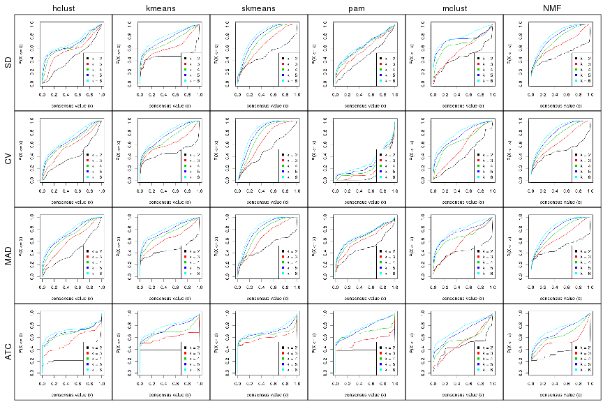
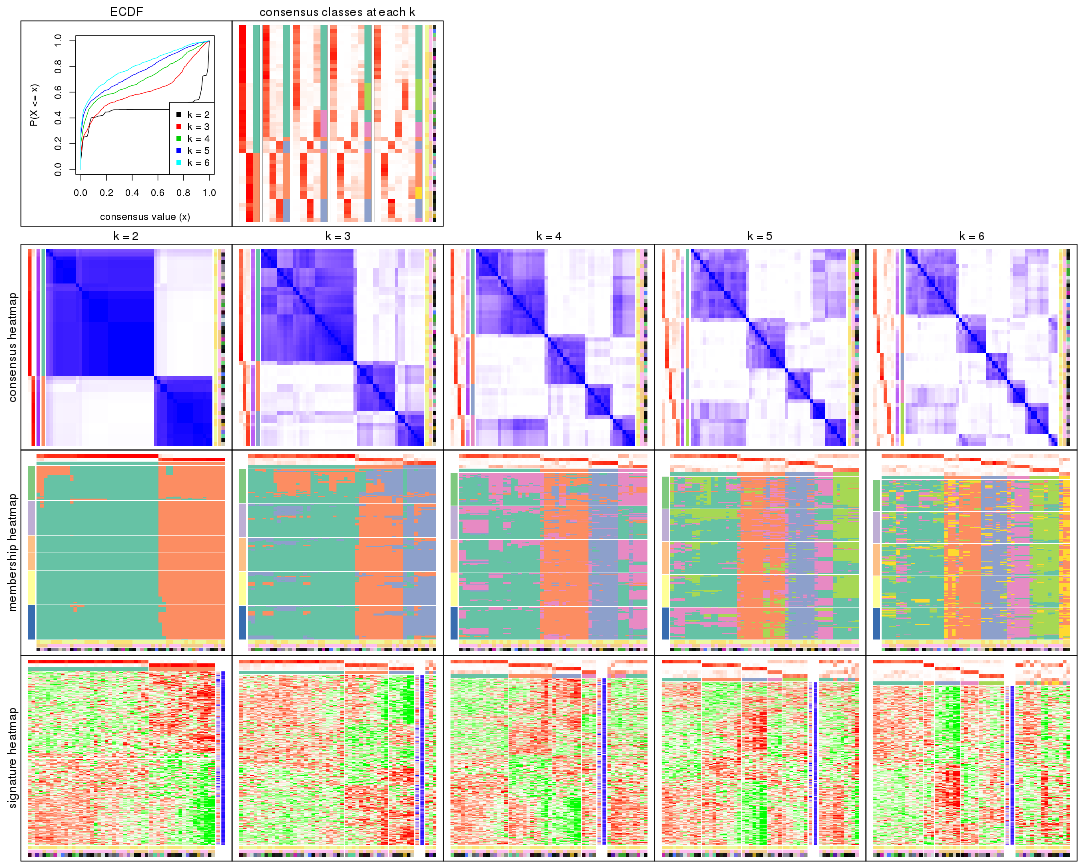
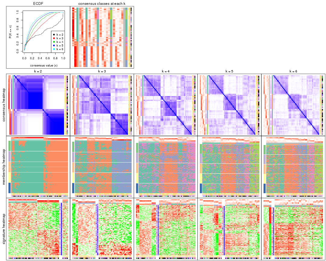
Cumulative distribution function curves of consensus matrix for all methods.
collect_plots(res_list, fun = plot_ecdf)
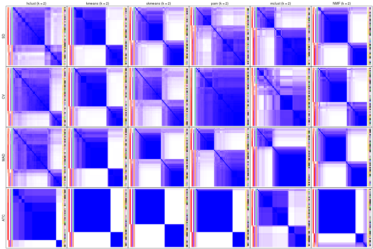
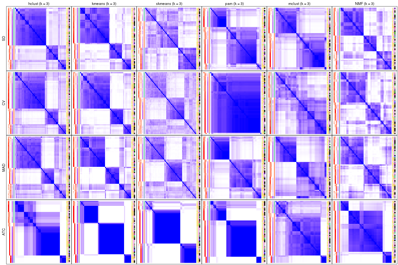
Consensus heatmaps for all methods. (What is a consensus heatmap?)
collect_plots(res_list, k = 2, fun = consensus_heatmap, mc.cores = 4)
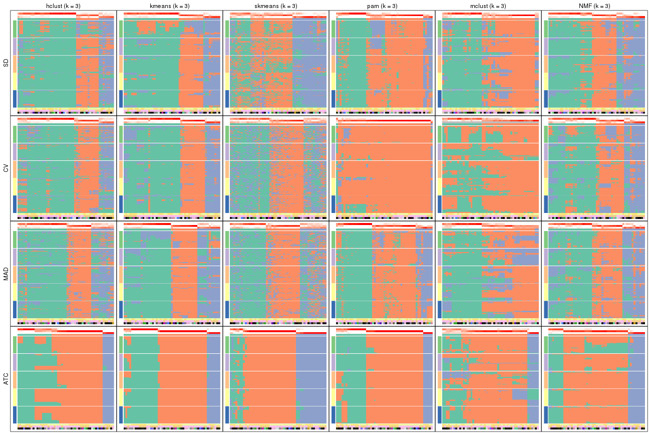
collect_plots(res_list, k = 3, fun = consensus_heatmap, mc.cores = 4)
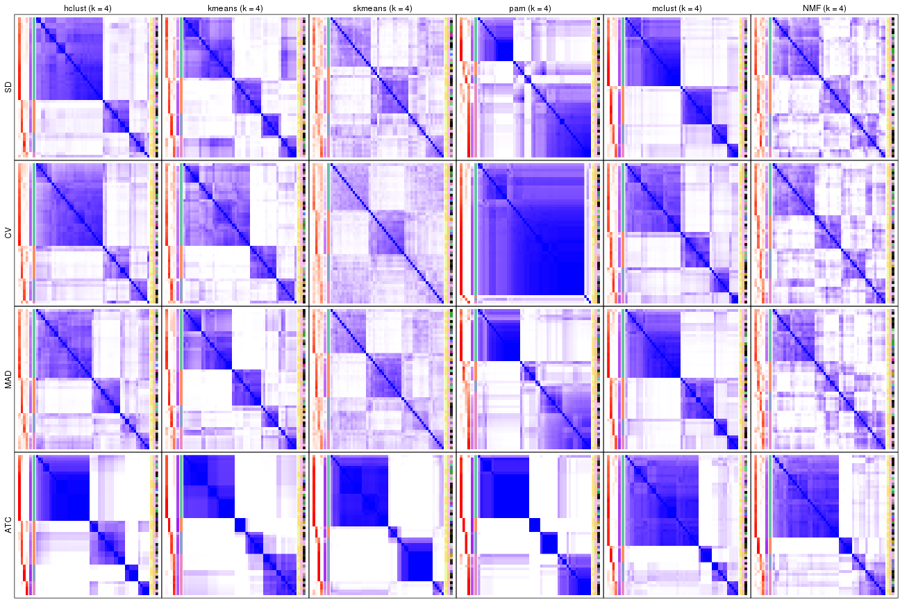
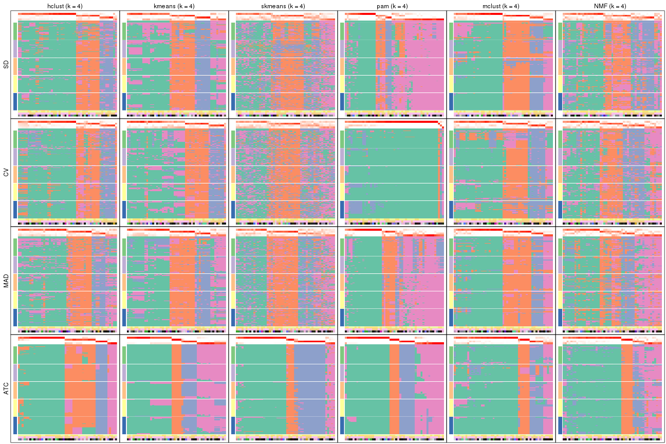
collect_plots(res_list, k = 4, fun = consensus_heatmap, mc.cores = 4)
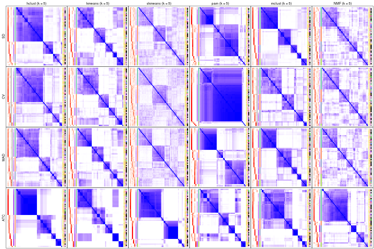
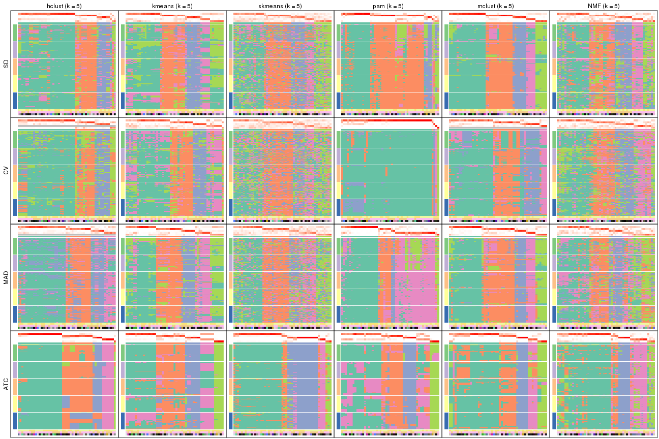
collect_plots(res_list, k = 5, fun = consensus_heatmap, mc.cores = 4)
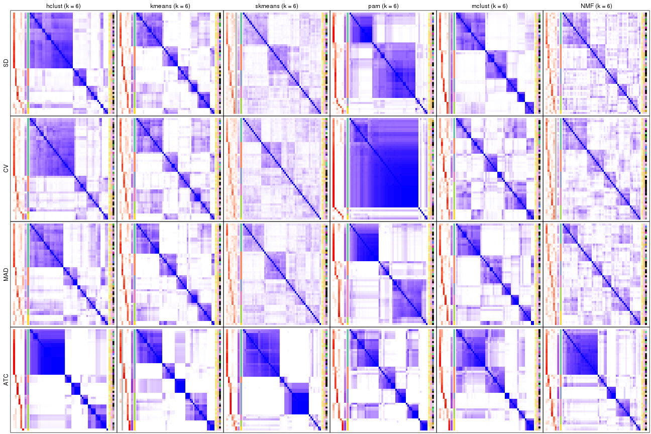
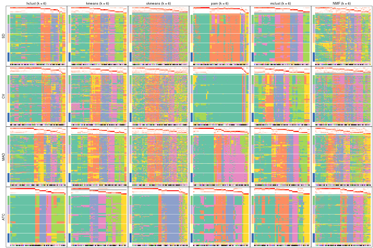
collect_plots(res_list, k = 6, fun = consensus_heatmap, mc.cores = 4)
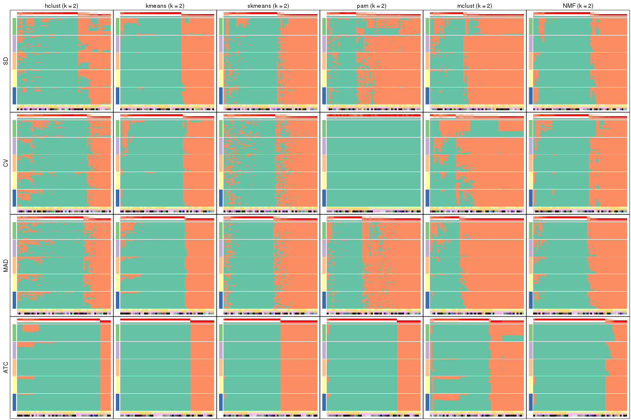
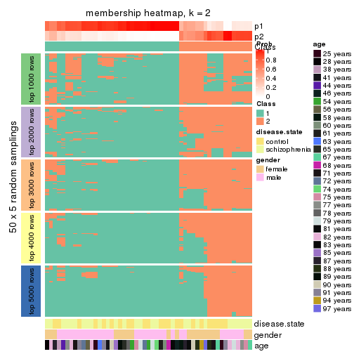
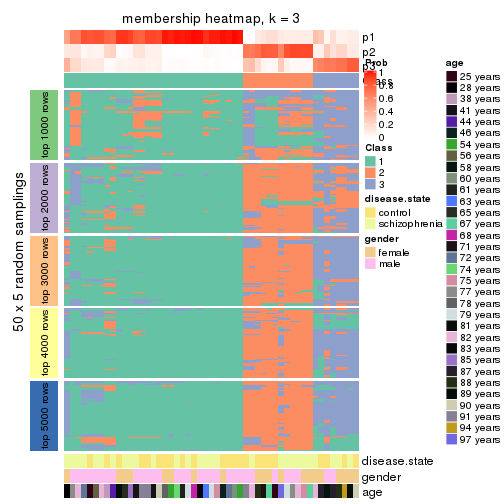
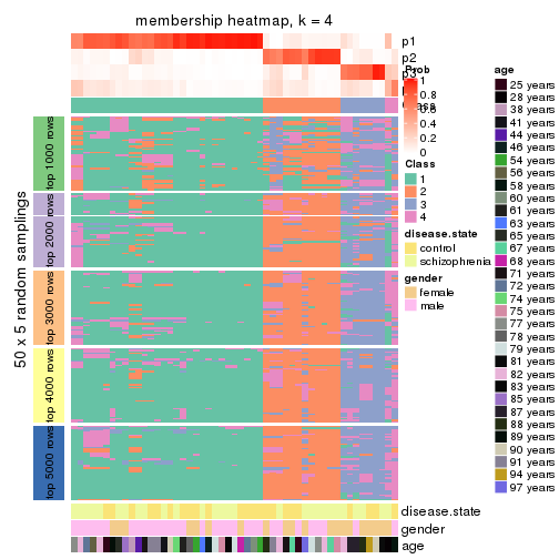
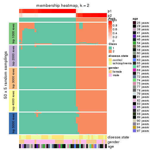
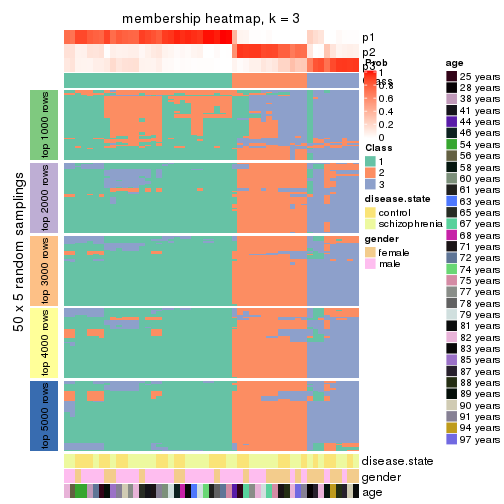
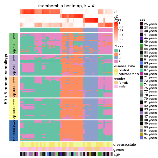
Membership heatmaps for all methods. (What is a membership heatmap?)
collect_plots(res_list, k = 2, fun = membership_heatmap, mc.cores = 4)
collect_plots(res_list, k = 3, fun = membership_heatmap, mc.cores = 4)
collect_plots(res_list, k = 4, fun = membership_heatmap, mc.cores = 4)
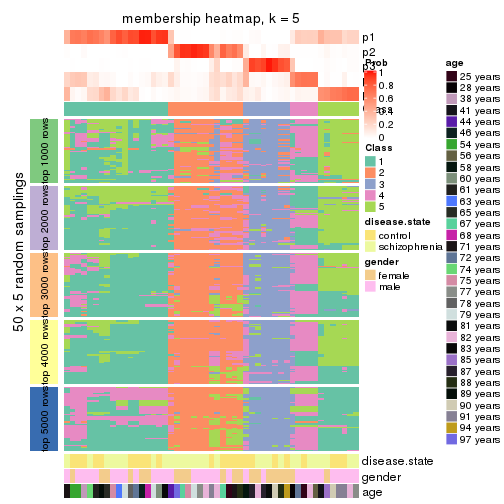
collect_plots(res_list, k = 5, fun = membership_heatmap, mc.cores = 4)
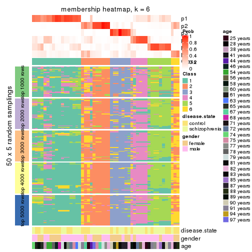
collect_plots(res_list, k = 6, fun = membership_heatmap, mc.cores = 4)
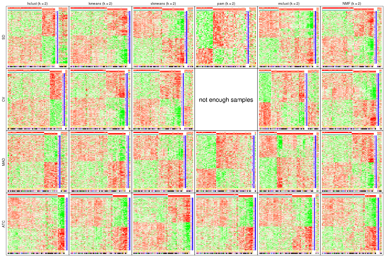
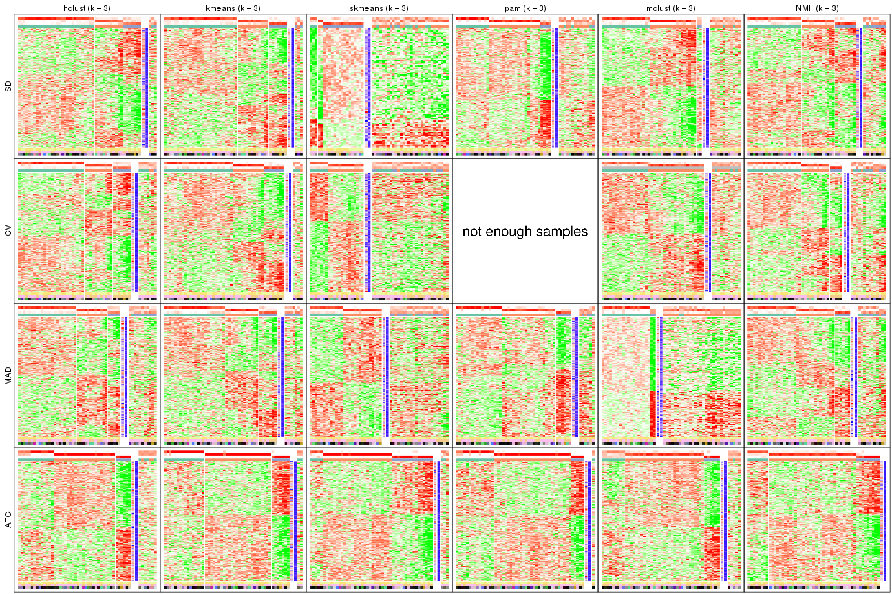
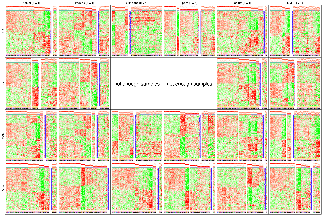
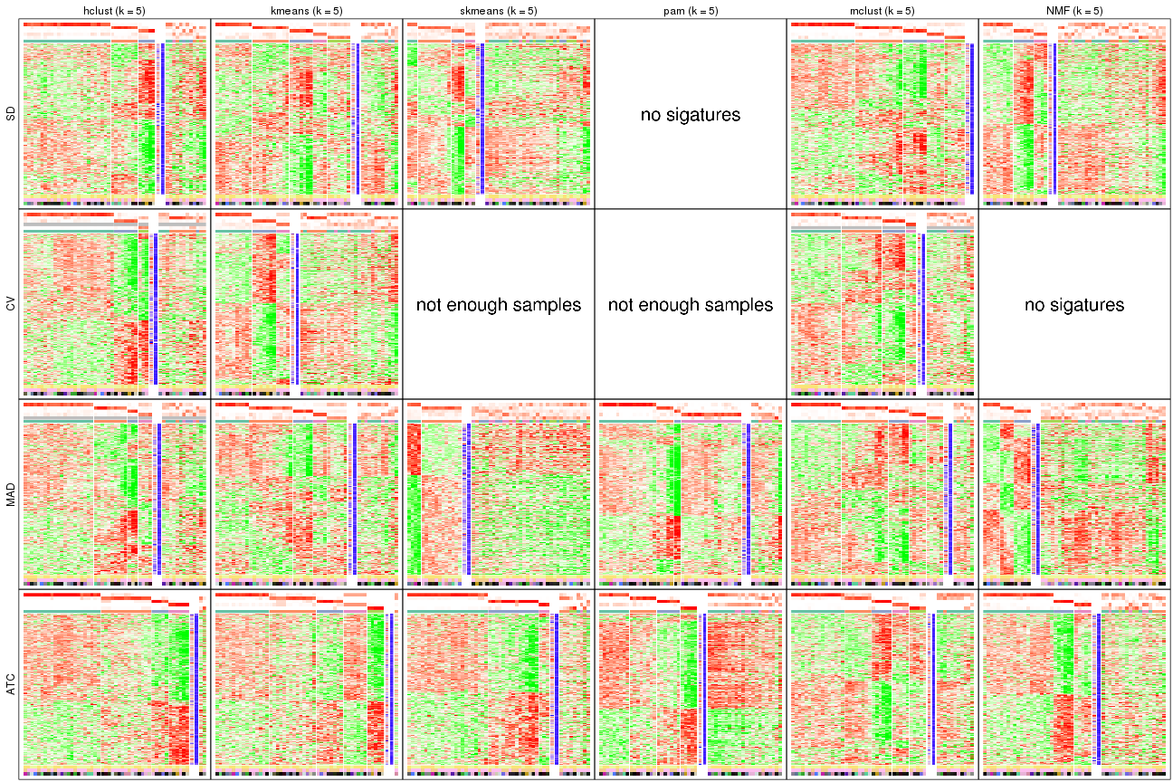
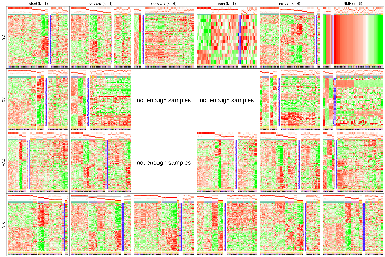
Signature heatmaps for all methods. (What is a signature heatmap?)
Note in following heatmaps, rows are scaled.
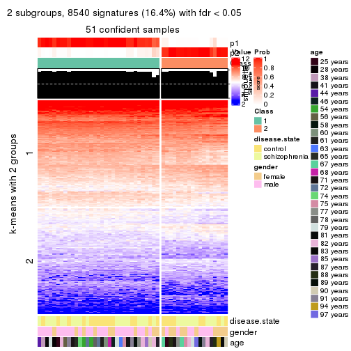
collect_plots(res_list, k = 2, fun = get_signatures, mc.cores = 4)
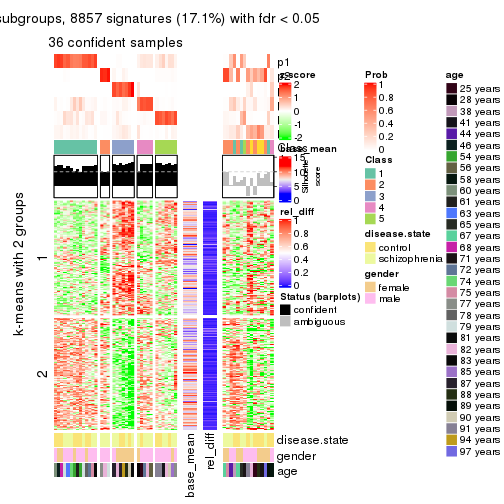
collect_plots(res_list, k = 3, fun = get_signatures, mc.cores = 4)
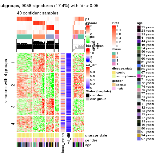
collect_plots(res_list, k = 4, fun = get_signatures, mc.cores = 4)
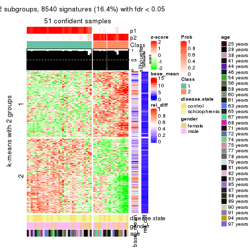
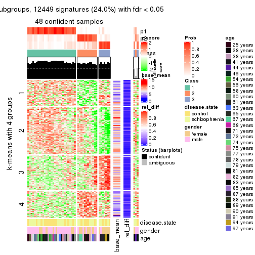
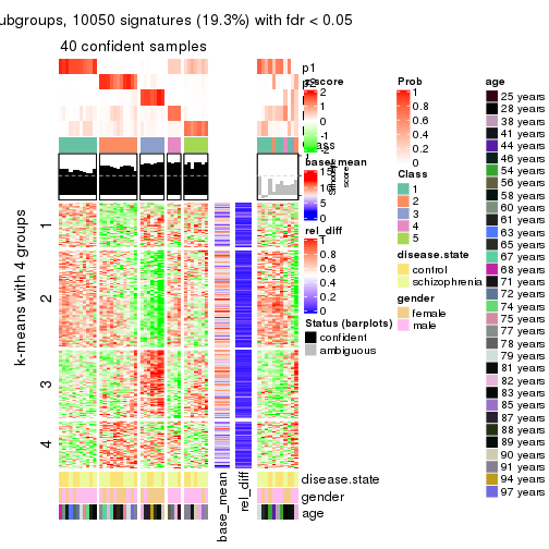
collect_plots(res_list, k = 5, fun = get_signatures, mc.cores = 4)
collect_plots(res_list, k = 6, fun = get_signatures, mc.cores = 4)
The statistics used for measuring the stability of consensus partitioning. (How are they defined?)
get_stats(res_list, k = 2)
#>             k 1-PAC mean_silhouette concordance area_increased  Rand Jaccard
#> SD:NMF      2 0.725           0.845       0.938          0.489 0.514   0.514
#> CV:NMF      2 0.642           0.858       0.930          0.494 0.506   0.506
#> MAD:NMF     2 0.729           0.848       0.941          0.496 0.500   0.500
#> ATC:NMF     2 0.878           0.929       0.966          0.336 0.633   0.633
#> SD:skmeans  2 0.566           0.789       0.911          0.504 0.500   0.500
#> CV:skmeans  2 0.331           0.748       0.870          0.506 0.495   0.495
#> MAD:skmeans 2 0.676           0.816       0.924          0.508 0.492   0.492
#> ATC:skmeans 2 1.000           0.996       0.998          0.487 0.514   0.514
#> SD:mclust   2 0.540           0.843       0.915          0.452 0.534   0.534
#> CV:mclust   2 0.235           0.656       0.791          0.412 0.594   0.594
#> MAD:mclust  2 0.691           0.898       0.946          0.421 0.561   0.561
#> ATC:mclust  2 0.595           0.866       0.922          0.457 0.523   0.523
#> SD:kmeans   2 0.974           0.950       0.971          0.469 0.534   0.534
#> CV:kmeans   2 0.834           0.904       0.954          0.464 0.547   0.547
#> MAD:kmeans  2 0.773           0.906       0.953          0.457 0.561   0.561
#> ATC:kmeans  2 1.000           1.000       1.000          0.388 0.613   0.613
#> SD:pam      2 0.279           0.747       0.861          0.458 0.561   0.561
#> CV:pam      2 0.536           0.000       0.935          0.114 1.000   1.000
#> MAD:pam     2 0.506           0.839       0.918          0.487 0.523   0.523
#> ATC:pam     2 1.000           0.985       0.993          0.394 0.613   0.613
#> SD:hclust   2 0.277           0.733       0.862          0.432 0.534   0.534
#> CV:hclust   2 0.412           0.797       0.883          0.413 0.613   0.613
#> MAD:hclust  2 0.401           0.725       0.867          0.429 0.576   0.576
#> ATC:hclust  2 0.785           0.943       0.965          0.252 0.788   0.788
get_stats(res_list, k = 3)
#>             k 1-PAC mean_silhouette concordance area_increased  Rand Jaccard
#> SD:NMF      3 0.449           0.681       0.824          0.349 0.740   0.534
#> CV:NMF      3 0.349           0.555       0.770          0.326 0.808   0.637
#> MAD:NMF     3 0.395           0.605       0.793          0.331 0.755   0.550
#> ATC:NMF     3 0.559           0.873       0.895          0.568 0.834   0.742
#> SD:skmeans  3 0.286           0.473       0.701          0.329 0.740   0.528
#> CV:skmeans  3 0.176           0.398       0.653          0.327 0.787   0.592
#> MAD:skmeans 3 0.271           0.476       0.707          0.320 0.758   0.544
#> ATC:skmeans 3 0.897           0.890       0.948          0.207 0.875   0.760
#> SD:mclust   3 0.356           0.533       0.795          0.272 0.843   0.728
#> CV:mclust   3 0.184           0.566       0.647          0.369 0.758   0.640
#> MAD:mclust  3 0.308           0.256       0.699          0.371 0.776   0.640
#> ATC:mclust  3 0.337           0.684       0.805          0.127 0.840   0.733
#> SD:kmeans   3 0.514           0.762       0.823          0.320 0.827   0.689
#> CV:kmeans   3 0.565           0.782       0.862          0.343 0.853   0.736
#> MAD:kmeans  3 0.514           0.715       0.824          0.405 0.766   0.595
#> ATC:kmeans  3 0.912           0.910       0.965          0.541 0.666   0.501
#> SD:pam      3 0.379           0.609       0.834          0.256 0.882   0.790
#> CV:pam      3 0.523           0.806       0.918          0.506 0.922   0.922
#> MAD:pam     3 0.429           0.713       0.855          0.279 0.838   0.690
#> ATC:pam     3 0.889           0.887       0.952          0.360 0.730   0.593
#> SD:hclust   3 0.285           0.741       0.824          0.314 0.885   0.789
#> CV:hclust   3 0.336           0.694       0.811          0.404 0.812   0.693
#> MAD:hclust  3 0.279           0.629       0.775          0.414 0.760   0.595
#> ATC:hclust  3 0.681           0.742       0.891          1.173 0.619   0.516
get_stats(res_list, k = 4)
#>             k 1-PAC mean_silhouette concordance area_increased  Rand Jaccard
#> SD:NMF      4 0.389           0.367       0.633         0.1241 0.845   0.608
#> CV:NMF      4 0.385           0.459       0.682         0.1365 0.821   0.551
#> MAD:NMF     4 0.413           0.438       0.684         0.1289 0.800   0.506
#> ATC:NMF     4 0.517           0.728       0.830         0.2120 0.771   0.588
#> SD:skmeans  4 0.302           0.351       0.583         0.1243 0.843   0.593
#> CV:skmeans  4 0.248           0.278       0.542         0.1236 0.835   0.566
#> MAD:skmeans 4 0.310           0.422       0.637         0.1219 0.873   0.642
#> ATC:skmeans 4 0.890           0.863       0.937         0.0999 0.945   0.867
#> SD:mclust   4 0.613           0.804       0.839         0.1782 0.728   0.489
#> CV:mclust   4 0.408           0.673       0.755         0.1945 0.692   0.461
#> MAD:mclust  4 0.597           0.773       0.849         0.1767 0.703   0.458
#> ATC:mclust  4 0.534           0.813       0.872         0.1322 0.921   0.848
#> SD:kmeans   4 0.589           0.602       0.746         0.1492 0.867   0.679
#> CV:kmeans   4 0.495           0.605       0.738         0.1376 0.991   0.978
#> MAD:kmeans  4 0.531           0.627       0.753         0.1370 0.893   0.716
#> ATC:kmeans  4 0.729           0.879       0.908         0.1465 0.844   0.636
#> SD:pam      4 0.426           0.575       0.821         0.0899 0.927   0.837
#> CV:pam      4 0.497           0.726       0.904         0.3720 0.962   0.959
#> MAD:pam     4 0.490           0.580       0.806         0.0874 0.953   0.871
#> ATC:pam     4 0.892           0.884       0.950         0.2765 0.780   0.548
#> SD:hclust   4 0.507           0.683       0.809         0.1230 0.970   0.932
#> CV:hclust   4 0.326           0.521       0.763         0.1179 0.991   0.978
#> MAD:hclust  4 0.379           0.570       0.714         0.1359 0.947   0.859
#> ATC:hclust  4 0.691           0.822       0.910         0.2279 0.862   0.685
get_stats(res_list, k = 5)
#>             k 1-PAC mean_silhouette concordance area_increased  Rand Jaccard
#> SD:NMF      5 0.442           0.427       0.648         0.0702 0.874   0.604
#> CV:NMF      5 0.447           0.346       0.605         0.0679 0.931   0.757
#> MAD:NMF     5 0.443           0.307       0.574         0.0680 0.896   0.644
#> ATC:NMF     5 0.553           0.563       0.789         0.1044 0.915   0.794
#> SD:skmeans  5 0.388           0.406       0.576         0.0639 0.910   0.688
#> CV:skmeans  5 0.337           0.265       0.499         0.0649 0.907   0.676
#> MAD:skmeans 5 0.366           0.378       0.581         0.0649 0.925   0.725
#> ATC:skmeans 5 0.774           0.771       0.889         0.0672 0.974   0.929
#> SD:mclust   5 0.697           0.852       0.885         0.1041 0.911   0.730
#> CV:mclust   5 0.495           0.563       0.701         0.1179 0.941   0.831
#> MAD:mclust  5 0.636           0.725       0.827         0.1067 0.860   0.613
#> ATC:mclust  5 0.512           0.632       0.806         0.1969 0.785   0.559
#> SD:kmeans   5 0.588           0.630       0.696         0.0772 0.871   0.598
#> CV:kmeans   5 0.467           0.377       0.660         0.0733 0.836   0.622
#> MAD:kmeans  5 0.621           0.595       0.740         0.0675 0.904   0.675
#> ATC:kmeans  5 0.681           0.810       0.800         0.0941 0.912   0.717
#> SD:pam      5 0.374           0.558       0.804         0.0364 0.953   0.884
#> CV:pam      5 0.537           0.674       0.897         0.2067 0.963   0.958
#> MAD:pam     5 0.521           0.616       0.820         0.0341 0.997   0.990
#> ATC:pam     5 0.628           0.536       0.743         0.1020 0.861   0.602
#> SD:hclust   5 0.542           0.584       0.793         0.0552 0.990   0.975
#> CV:hclust   5 0.384           0.584       0.727         0.0524 0.983   0.959
#> MAD:hclust  5 0.449           0.541       0.687         0.0667 1.000   1.000
#> ATC:hclust  5 0.700           0.805       0.891         0.0268 0.982   0.945
get_stats(res_list, k = 6)
#>             k 1-PAC mean_silhouette concordance area_increased  Rand Jaccard
#> SD:NMF      6 0.473           0.300       0.561         0.0430 0.947   0.776
#> CV:NMF      6 0.487           0.331       0.550         0.0425 0.937   0.753
#> MAD:NMF     6 0.496           0.345       0.563         0.0441 0.846   0.417
#> ATC:NMF     6 0.593           0.595       0.792         0.0594 0.891   0.694
#> SD:skmeans  6 0.475           0.365       0.560         0.0421 0.974   0.886
#> CV:skmeans  6 0.396           0.239       0.479         0.0438 0.911   0.645
#> MAD:skmeans 6 0.455           0.308       0.542         0.0417 0.937   0.735
#> ATC:skmeans 6 0.703           0.709       0.844         0.0448 0.972   0.918
#> SD:mclust   6 0.678           0.752       0.799         0.0666 1.000   1.000
#> CV:mclust   6 0.564           0.371       0.654         0.0616 0.836   0.493
#> MAD:mclust  6 0.590           0.524       0.752         0.0588 0.943   0.775
#> ATC:mclust  6 0.613           0.612       0.797         0.0793 0.849   0.559
#> SD:kmeans   6 0.611           0.565       0.749         0.0550 0.948   0.781
#> CV:kmeans   6 0.509           0.412       0.624         0.0494 0.892   0.634
#> MAD:kmeans  6 0.640           0.494       0.713         0.0496 0.954   0.792
#> ATC:kmeans  6 0.710           0.757       0.802         0.0572 0.976   0.900
#> SD:pam      6 0.394           0.590       0.809         0.0195 0.995   0.986
#> CV:pam      6 0.499           0.649       0.886         0.1486 0.928   0.915
#> MAD:pam     6 0.528           0.564       0.800         0.0196 0.968   0.899
#> ATC:pam     6 0.644           0.528       0.772         0.0308 0.853   0.524
#> SD:hclust   6 0.551           0.563       0.766         0.0534 0.938   0.847
#> CV:hclust   6 0.438           0.475       0.678         0.0582 0.963   0.908
#> MAD:hclust  6 0.457           0.359       0.602         0.0422 0.909   0.724
#> ATC:hclust  6 0.743           0.797       0.884         0.0519 0.962   0.879
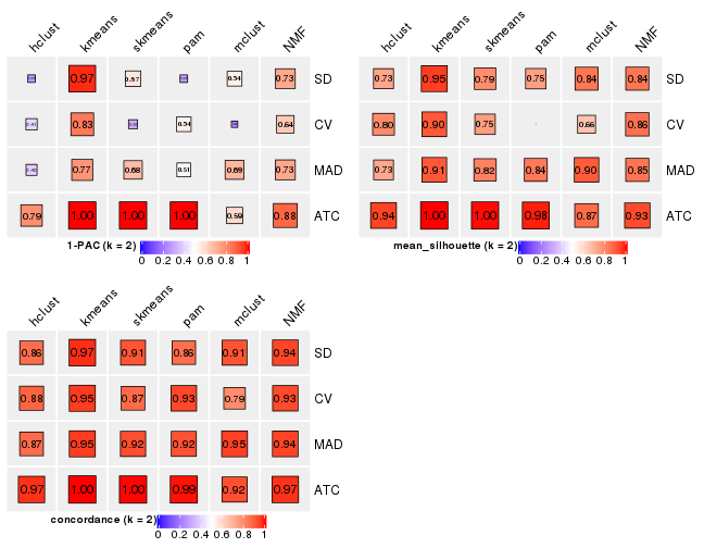
Following heatmap plots the partition for each combination of methods and the lightness correspond to the silhouette scores for samples in each method. On top the consensus subgroup is inferred from all methods by taking the mean silhouette scores as weight.
collect_stats(res_list, k = 2)
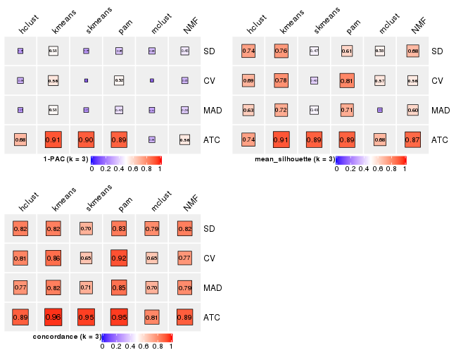
collect_stats(res_list, k = 3)
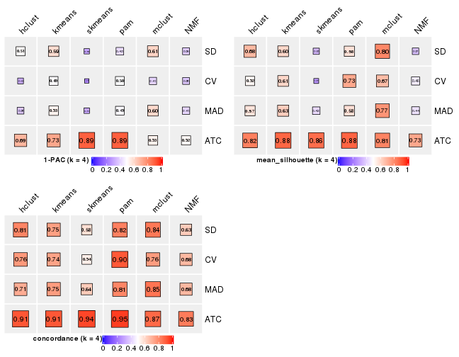
collect_stats(res_list, k = 4)
collect_stats(res_list, k = 5)
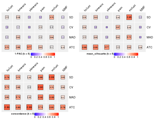
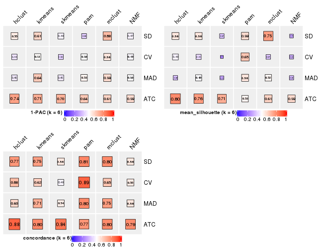
collect_stats(res_list, k = 6)
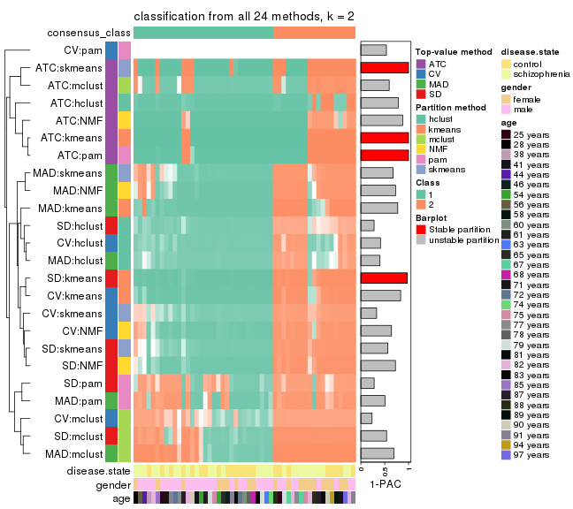
Collect partitions from all methods:
collect_classes(res_list, k = 2)
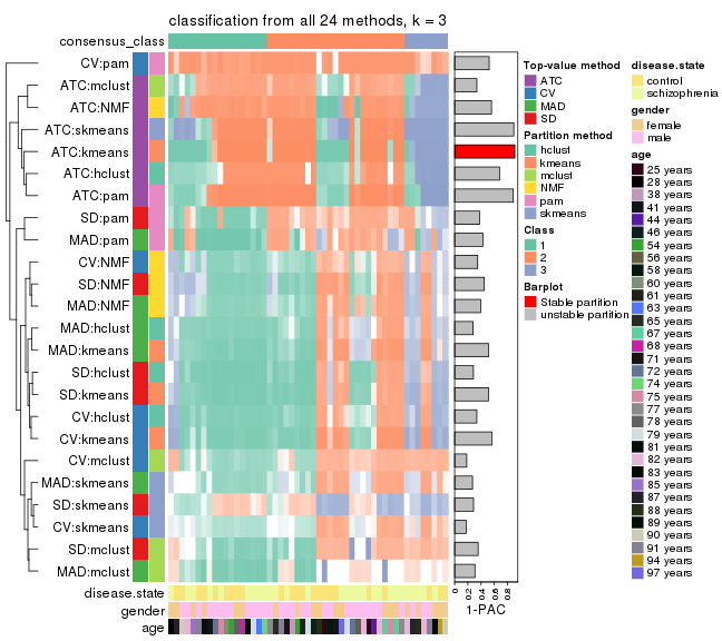
collect_classes(res_list, k = 3)
collect_classes(res_list, k = 4)
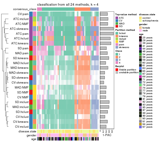
collect_classes(res_list, k = 5)
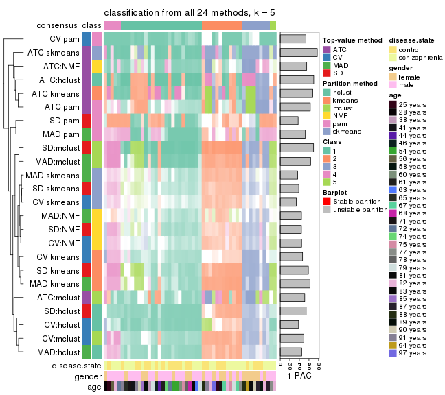
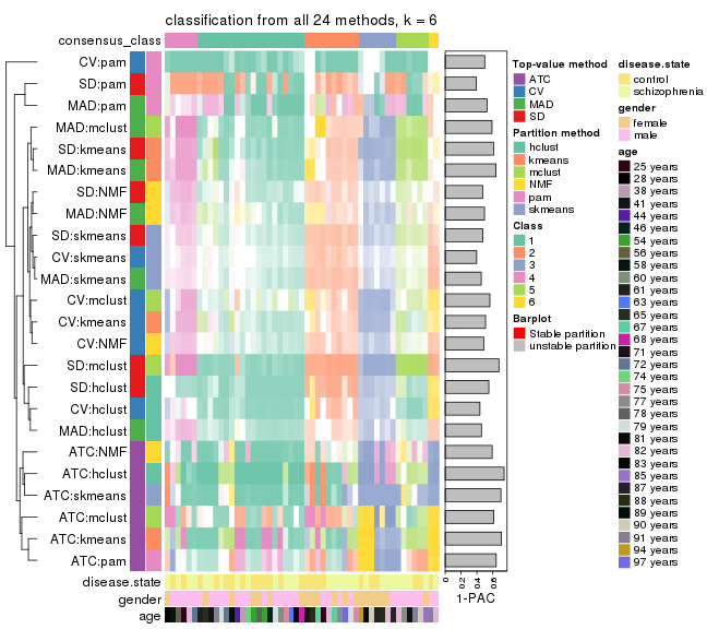
collect_classes(res_list, k = 6)
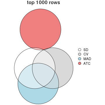
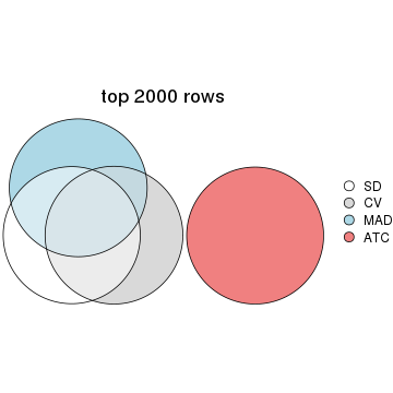
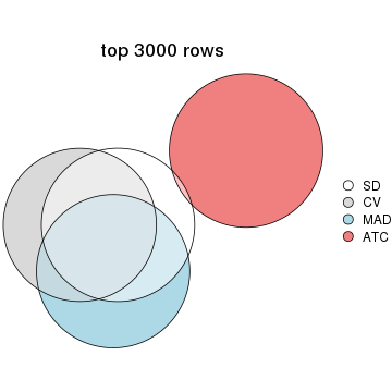
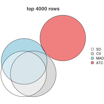
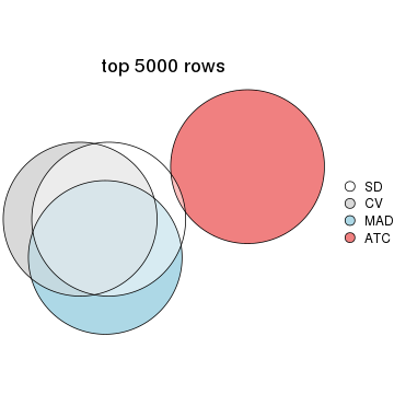
Overlap of top rows from different top-row methods:
top_rows_overlap(res_list, top_n = 1000, method = "euler")
top_rows_overlap(res_list, top_n = 2000, method = "euler")
top_rows_overlap(res_list, top_n = 3000, method = "euler")
top_rows_overlap(res_list, top_n = 4000, method = "euler")
top_rows_overlap(res_list, top_n = 5000, method = "euler")
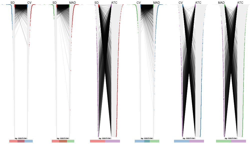
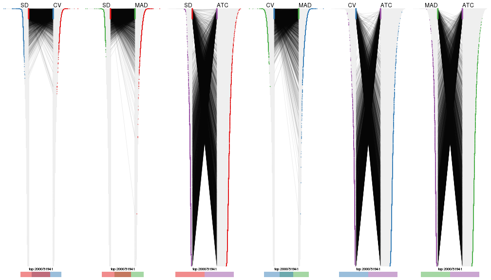
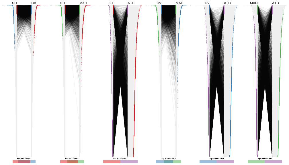
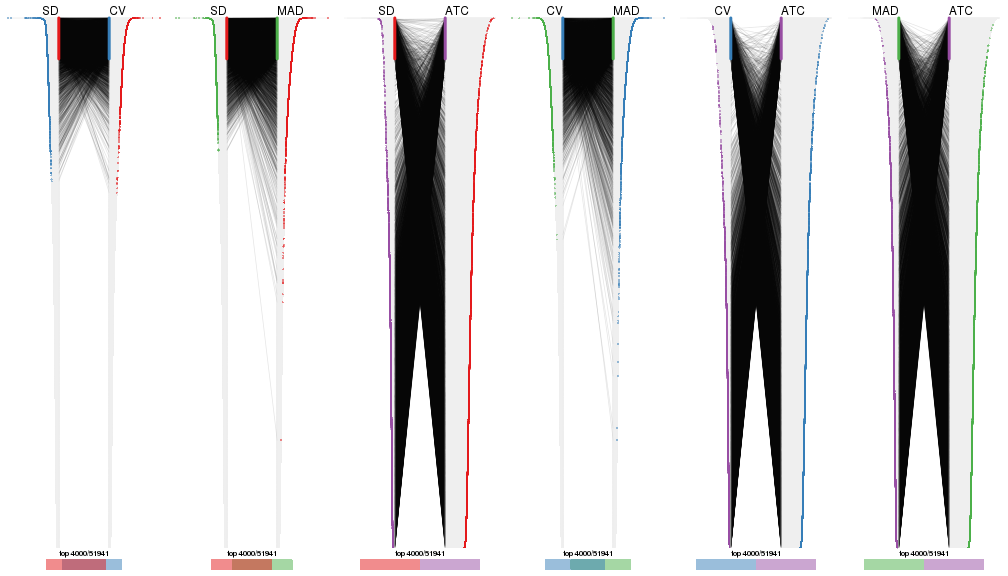
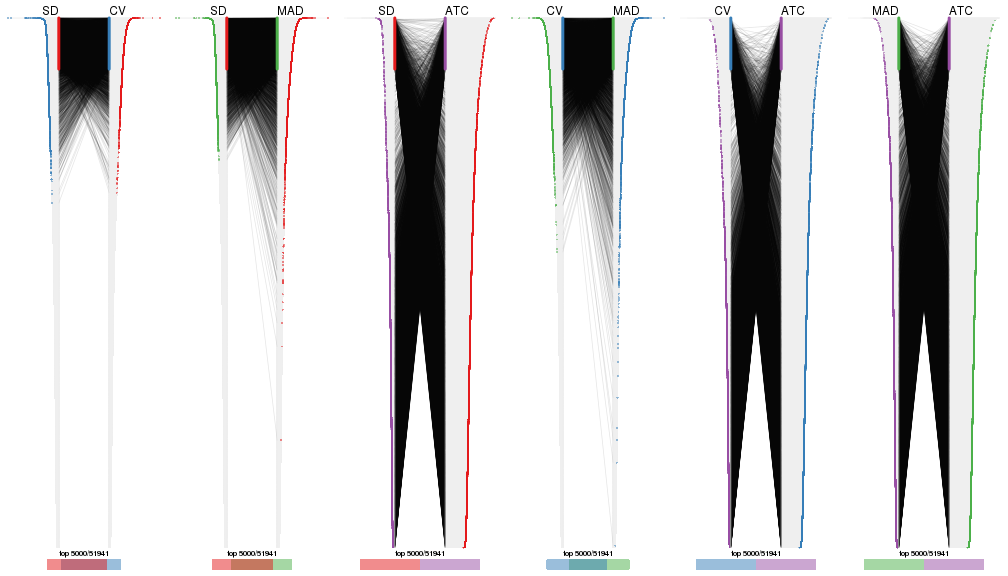
Also visualize the correspondance of rankings between different top-row methods:
top_rows_overlap(res_list, top_n = 1000, method = "correspondance")
top_rows_overlap(res_list, top_n = 2000, method = "correspondance")
top_rows_overlap(res_list, top_n = 3000, method = "correspondance")
top_rows_overlap(res_list, top_n = 4000, method = "correspondance")
top_rows_overlap(res_list, top_n = 5000, method = "correspondance")
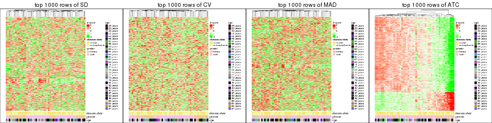
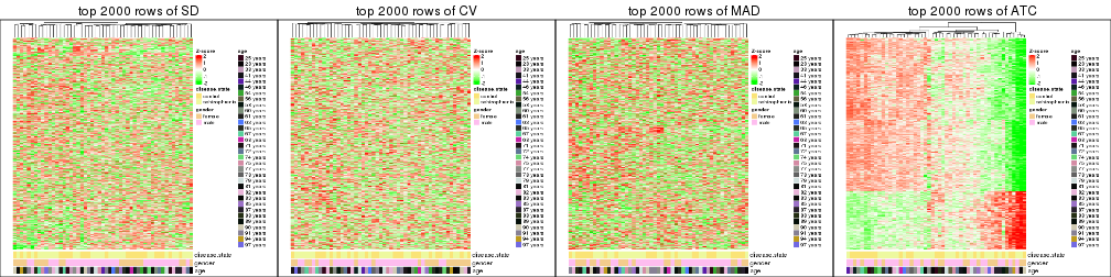
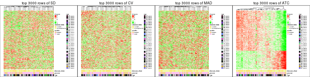
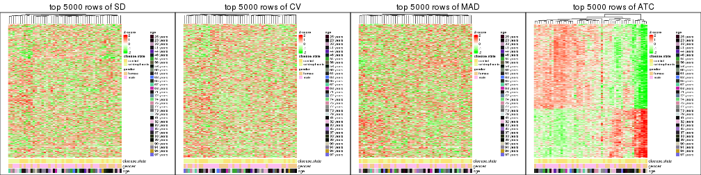
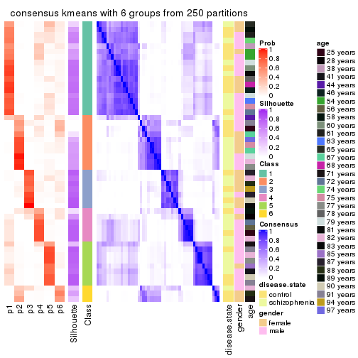
Heatmaps of the top rows:
top_rows_heatmap(res_list, top_n = 1000)
top_rows_heatmap(res_list, top_n = 2000)
top_rows_heatmap(res_list, top_n = 3000)
top_rows_heatmap(res_list, top_n = 4000)
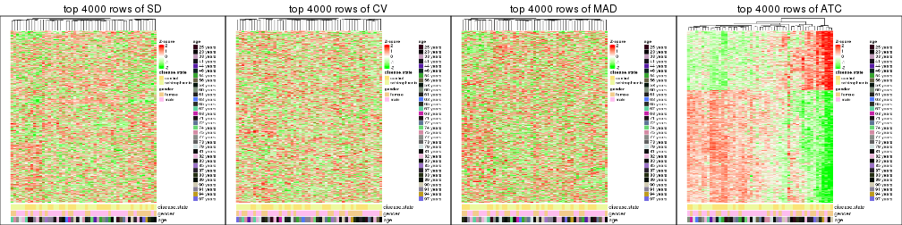
top_rows_heatmap(res_list, top_n = 5000)
Test correlation between subgroups and known annotations. If the known annotation is numeric, one-way ANOVA test is applied, and if the known annotation is discrete, chi-squared contingency table test is applied.
test_to_known_factors(res_list, k = 2)
#>              n disease.state(p) gender(p) age(p) k
#> SD:NMF      47            0.853    0.1076  0.707 2
#> CV:NMF      49            0.432    0.1626  0.657 2
#> MAD:NMF     47            0.796    0.6100  0.723 2
#> ATC:NMF     49            1.000    0.0811  0.389 2
#> SD:skmeans  46            0.526    0.0252  0.553 2
#> CV:skmeans  43            0.836    0.1129  0.569 2
#> MAD:skmeans 45            0.443    0.4646  0.552 2
#> ATC:skmeans 51            0.782    0.1186  0.280 2
#> SD:mclust   49            0.398    0.6096  0.256 2
#> CV:mclust   41            0.132    0.6727  0.397 2
#> MAD:mclust  49            0.420    0.9849  0.202 2
#> ATC:mclust  48            1.000    0.0696  0.254 2
#> SD:kmeans   51            1.000    0.1429  0.729 2
#> CV:kmeans   49            1.000    0.1603  0.787 2
#> MAD:kmeans  50            0.932    0.3751  0.787 2
#> ATC:kmeans  51            1.000    0.1139  0.405 2
#> SD:pam      45            0.243    1.0000  0.278 2
#> CV:pam       0               NA        NA     NA 2
#> MAD:pam     50            0.126    0.6738  0.353 2
#> ATC:pam     51            1.000    0.1139  0.405 2
#> SD:hclust   43            1.000    0.2478  0.806 2
#> CV:hclust   49            1.000    0.4816  0.814 2
#> MAD:hclust  45            1.000    0.5015  0.790 2
#> ATC:hclust  51            1.000    0.3072  0.706 2
test_to_known_factors(res_list, k = 3)
#>              n disease.state(p) gender(p) age(p) k
#> SD:NMF      42           0.4149   0.05908  0.509 3
#> CV:NMF      37           0.3176   0.00299  0.460 3
#> MAD:NMF     40           0.2343   0.10893  0.342 3
#> ATC:NMF     51           0.4736   0.12254  0.618 3
#> SD:skmeans  21           0.3181   0.08535  0.563 3
#> CV:skmeans  21           1.0000   0.26609  0.343 3
#> MAD:skmeans 28           0.6840   0.63759  0.405 3
#> ATC:skmeans 48           0.7973   0.15716  0.219 3
#> SD:mclust   39           0.7151   0.16019  0.688 3
#> CV:mclust   40           0.5454   0.09671  0.350 3
#> MAD:mclust  21           0.6885   1.00000  0.279 3
#> ATC:mclust  46           0.9734   0.05219  0.470 3
#> SD:kmeans   48           0.9146   0.00796  0.580 3
#> CV:kmeans   47           0.8427   0.00126  0.515 3
#> MAD:kmeans  44           0.2340   0.12160  0.593 3
#> ATC:kmeans  49           0.9449   0.10928  0.794 3
#> SD:pam      37           0.0858   0.08906  0.551 3
#> CV:pam      46               NA        NA     NA 3
#> MAD:pam     45           0.0243   0.29259  0.675 3
#> ATC:pam     50           0.6847   0.12496  0.512 3
#> SD:hclust   48           0.9831   0.00741  0.638 3
#> CV:hclust   44           0.9309   0.00206  0.603 3
#> MAD:hclust  40           0.7874   0.33119  0.465 3
#> ATC:hclust  44           0.7976   0.11178  0.679 3
test_to_known_factors(res_list, k = 4)
#>              n disease.state(p) gender(p) age(p) k
#> SD:NMF      22           0.5836  0.017061  0.689 4
#> CV:NMF      27           0.3503  0.013396  0.862 4
#> MAD:NMF     23           0.1432  0.097482  0.302 4
#> ATC:NMF     43           0.9874  0.445109  0.374 4
#> SD:skmeans  18           0.6247  0.110494  0.476 4
#> CV:skmeans  12               NA        NA     NA 4
#> MAD:skmeans 23           0.7747  0.179231  0.543 4
#> ATC:skmeans 48           0.6508  0.207494  0.317 4
#> SD:mclust   49           0.5095  0.041305  0.523 4
#> CV:mclust   45           0.9466  0.001523  0.841 4
#> MAD:mclust  48           0.5563  0.076998  0.521 4
#> ATC:mclust  50           0.3495  0.147988  0.429 4
#> SD:kmeans   40           0.8734  0.057068  0.658 4
#> CV:kmeans   41           0.7283  0.000512  0.579 4
#> MAD:kmeans  39           0.7676  0.046121  0.558 4
#> ATC:kmeans  51           0.8347  0.297258  0.486 4
#> SD:pam      37           0.0999  0.155319  0.841 4
#> CV:pam      44               NA        NA     NA 4
#> MAD:pam     37           0.0208  0.051718  0.446 4
#> ATC:pam     49           0.8483  0.271562  0.463 4
#> SD:hclust   47           0.9341  0.026046  0.546 4
#> CV:hclust   34           1.0000  0.001823  0.471 4
#> MAD:hclust  40           0.7929  0.200321  0.592 4
#> ATC:hclust  46           0.8476  0.206226  0.355 4
test_to_known_factors(res_list, k = 5)
#>              n disease.state(p) gender(p) age(p) k
#> SD:NMF      19           0.9711  0.000506  0.466 5
#> CV:NMF      10           0.3541  0.061999  0.735 5
#> MAD:NMF     14           0.0541  0.363815  0.304 5
#> ATC:NMF     32           0.8835  0.341194  0.603 5
#> SD:skmeans  21           0.6836  0.286586  0.633 5
#> CV:skmeans   9               NA        NA     NA 5
#> MAD:skmeans 17           0.3194  0.377585  0.201 5
#> ATC:skmeans 43           0.5934  0.133109  0.165 5
#> SD:mclust   51           0.5736  0.062453  0.543 5
#> CV:mclust   37           0.7094  0.001818  0.762 5
#> MAD:mclust  45           0.5521  0.171855  0.598 5
#> ATC:mclust  40           0.3673  0.311273  0.128 5
#> SD:kmeans   40           0.8977  0.014596  0.510 5
#> CV:kmeans   22           0.5884  0.001360  0.566 5
#> MAD:kmeans  39           0.9095  0.091141  0.475 5
#> ATC:kmeans  50           0.1630  0.474943  0.522 5
#> SD:pam      34           0.0921  0.713586  0.376 5
#> CV:pam      42               NA        NA     NA 5
#> MAD:pam     42           0.1362  0.055607  0.402 5
#> ATC:pam     30           0.4756  0.834763  0.258 5
#> SD:hclust   39           0.7898  0.062116  0.387 5
#> CV:hclust   37           0.7841  0.001726  0.947 5
#> MAD:hclust  38           0.7341  0.180146  0.604 5
#> ATC:hclust  49           0.9530  0.286693  0.425 5
test_to_known_factors(res_list, k = 6)
#>              n disease.state(p) gender(p) age(p) k
#> SD:NMF       7           1.0000        NA  0.321 6
#> CV:NMF       9           0.8290   0.01111  0.353 6
#> MAD:NMF     10           0.7316   0.15335  0.298 6
#> ATC:NMF     35           0.9573   0.58607  0.355 6
#> SD:skmeans   8           0.5866   0.10093  0.512 6
#> CV:skmeans   3               NA        NA     NA 6
#> MAD:skmeans  7               NA        NA     NA 6
#> ATC:skmeans 41           0.7378   0.25206  0.443 6
#> SD:mclust   49           0.6310   0.06746  0.510 6
#> CV:mclust   16           0.3508   0.01000  0.418 6
#> MAD:mclust  34           0.2281   0.14187  0.542 6
#> ATC:mclust  39           0.6938   0.43853  0.272 6
#> SD:kmeans   36           0.3430   0.01867  0.551 6
#> CV:kmeans   16           0.6195   0.00976  0.666 6
#> MAD:kmeans  31           0.3483   0.05047  0.316 6
#> ATC:kmeans  45           0.1672   0.46599  0.504 6
#> SD:pam      37           0.0454   1.00000  0.296 6
#> CV:pam      39               NA        NA     NA 6
#> MAD:pam     35           0.0572   0.04111  0.651 6
#> ATC:pam     24           0.2597   0.87656  0.331 6
#> SD:hclust   36           0.9423   0.02647  0.434 6
#> CV:hclust   33           0.4692   0.05006  0.674 6
#> MAD:hclust  17           0.4316   0.15930  0.414 6
#> ATC:hclust  49           0.5752   0.09925  0.426 6
The object with results only for a single top-value method and a single partition method can be extracted as:
res = res_list["SD", "hclust"]
# you can also extract it by
# res = res_list["SD:hclust"]
A summary of res and all the functions that can be applied to it:
res
#> A 'ConsensusPartition' object with k = 2, 3, 4, 5, 6.
#>   On a matrix with 51941 rows and 51 columns.
#>   Top rows (1000, 2000, 3000, 4000, 5000) are extracted by 'SD' method.
#>   Subgroups are detected by 'hclust' method.
#>   Performed in total 1250 partitions by row resampling.
#>   Best k for subgroups seems to be 2.
#>
#> Following methods can be applied to this 'ConsensusPartition' object:
#>  [1] "cola_report"             "collect_classes"         "collect_plots"
#>  [4] "collect_stats"           "colnames"                "compare_signatures"
#>  [7] "consensus_heatmap"       "dimension_reduction"     "functional_enrichment"
#> [10] "get_anno_col"            "get_anno"                "get_classes"
#> [13] "get_consensus"           "get_matrix"              "get_membership"
#> [16] "get_param"               "get_signatures"          "get_stats"
#> [19] "is_best_k"               "is_stable_k"             "membership_heatmap"
#> [22] "ncol"                    "nrow"                    "plot_ecdf"
#> [25] "rownames"                "select_partition_number" "show"
#> [28] "suggest_best_k"          "test_to_known_factors"
collect_plots() function collects all the plots made from res for all k (number of partitions)
into one single page to provide an easy and fast comparison between different k.
collect_plots(res)
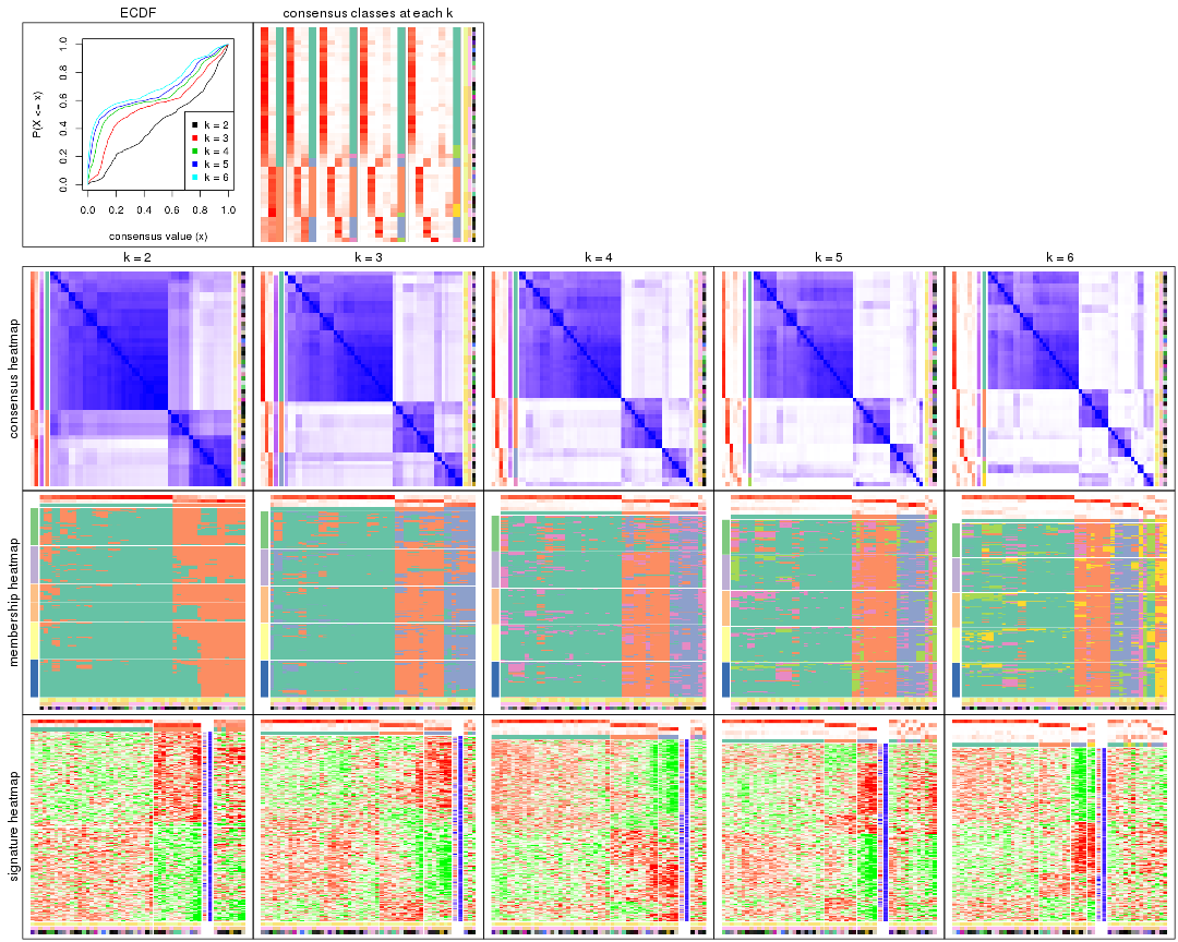
The plots are:
k and the heatmap of
predicted classes for each k.k.k.k.All the plots in panels can be made by individual functions and they are plotted later in this section.
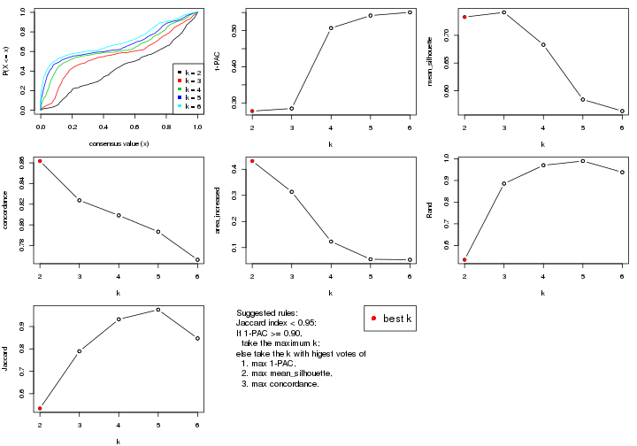
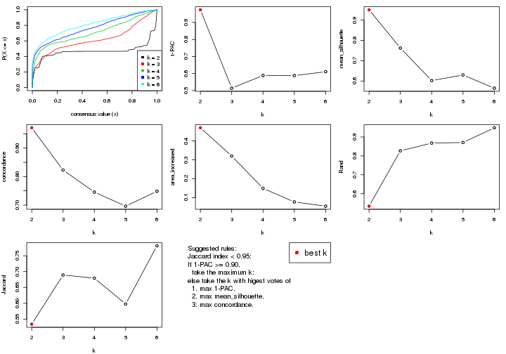
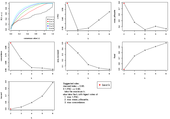
select_partition_number() produces several plots showing different
statistics for choosing “optimized” k. There are following statistics:
k;k, the area increased is defined as \(A_k - A_{k-1}\).The detailed explanations of these statistics can be found in the cola vignette.
Generally speaking, lower PAC score, higher mean silhouette score or higher
concordance corresponds to better partition. Rand index and Jaccard index
measure how similar the current partition is compared to partition with k-1.
If they are too similar, we won't accept k is better than k-1.
select_partition_number(res)
The numeric values for all these statistics can be obtained by get_stats().
get_stats(res)
#>   k 1-PAC mean_silhouette concordance area_increased  Rand Jaccard
#> 2 2 0.277           0.733       0.862         0.4316 0.534   0.534
#> 3 3 0.285           0.741       0.824         0.3136 0.885   0.789
#> 4 4 0.507           0.683       0.809         0.1230 0.970   0.932
#> 5 5 0.542           0.584       0.793         0.0552 0.990   0.975
#> 6 6 0.551           0.563       0.766         0.0534 0.938   0.847
suggest_best_k() suggests the best \(k\) based on these statistics. The rules are as follows:
suggest_best_k(res)
#> [1] 2
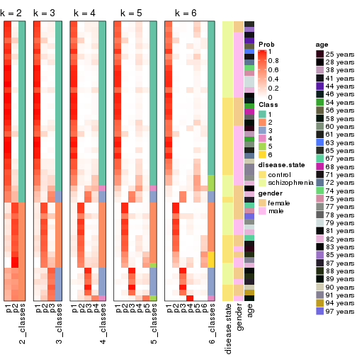
Following shows the table of the partitions (You need to click the show/hide
code output link to see it). The membership matrix (columns with name p*)
is inferred by
clue::cl_consensus()
function with the SE method. Basically the value in the membership matrix
represents the probability to belong to a certain group. The finall class
label for an item is determined with the group with highest probability it
belongs to.
In get_classes() function, the entropy is calculated from the membership
matrix and the silhouette score is calculated from the consensus matrix.
cbind(get_classes(res, k = 2), get_membership(res, k = 2))
#>           class entropy silhouette    p1    p2
#> GSM439800     1  0.8499      0.546 0.724 0.276
#> GSM439790     1  0.2603      0.880 0.956 0.044
#> GSM439827     2  0.5059      0.754 0.112 0.888
#> GSM439811     2  0.5178      0.754 0.116 0.884
#> GSM439795     2  0.9933      0.254 0.452 0.548
#> GSM439805     1  0.9491      0.348 0.632 0.368
#> GSM439781     1  0.3584      0.873 0.932 0.068
#> GSM439807     2  0.9635      0.419 0.388 0.612
#> GSM439820     2  0.8081      0.678 0.248 0.752
#> GSM439784     1  0.4161      0.862 0.916 0.084
#> GSM439824     1  0.8016      0.616 0.756 0.244
#> GSM439794     1  0.4161      0.851 0.916 0.084
#> GSM439809     1  0.2778      0.878 0.952 0.048
#> GSM439785     1  0.6438      0.799 0.836 0.164
#> GSM439803     1  0.3879      0.860 0.924 0.076
#> GSM439778     1  0.0376      0.882 0.996 0.004
#> GSM439791     1  0.1184      0.883 0.984 0.016
#> GSM439786     1  0.6048      0.794 0.852 0.148
#> GSM439828     2  0.5059      0.754 0.112 0.888
#> GSM439806     1  0.1184      0.882 0.984 0.016
#> GSM439815     1  0.0000      0.880 1.000 0.000
#> GSM439817     2  0.5629      0.752 0.132 0.868
#> GSM439796     1  0.4298      0.847 0.912 0.088
#> GSM439798     1  0.6343      0.788 0.840 0.160
#> GSM439821     2  0.0376      0.715 0.004 0.996
#> GSM439823     2  0.5294      0.754 0.120 0.880
#> GSM439813     1  0.0376      0.879 0.996 0.004
#> GSM439801     2  0.9993      0.124 0.484 0.516
#> GSM439810     1  0.0376      0.879 0.996 0.004
#> GSM439783     1  0.1633      0.884 0.976 0.024
#> GSM439826     2  0.7056      0.717 0.192 0.808
#> GSM439812     1  0.0376      0.879 0.996 0.004
#> GSM439818     2  0.6343      0.733 0.160 0.840
#> GSM439792     1  0.0938      0.883 0.988 0.012
#> GSM439802     1  0.9491      0.359 0.632 0.368
#> GSM439825     2  0.4939      0.735 0.108 0.892
#> GSM439780     1  0.2236      0.881 0.964 0.036
#> GSM439787     2  0.9922      0.266 0.448 0.552
#> GSM439808     2  0.9635      0.419 0.388 0.612
#> GSM439804     1  0.4562      0.839 0.904 0.096
#> GSM439822     2  0.6973      0.718 0.188 0.812
#> GSM439816     1  0.7528      0.671 0.784 0.216
#> GSM439789     1  0.0938      0.881 0.988 0.012
#> GSM439799     2  0.9491      0.451 0.368 0.632
#> GSM439814     1  0.0376      0.879 0.996 0.004
#> GSM439782     1  0.0376      0.882 0.996 0.004
#> GSM439779     1  0.1414      0.884 0.980 0.020
#> GSM439793     1  0.4298      0.860 0.912 0.088
#> GSM439788     1  0.3733      0.869 0.928 0.072
#> GSM439797     1  0.6623      0.790 0.828 0.172
#> GSM439819     2  0.0672      0.717 0.008 0.992
cbind(get_classes(res, k = 3), get_membership(res, k = 3))
#>           class entropy silhouette    p1    p2    p3
#> GSM439800     1  0.8865     -0.181 0.476 0.120 0.404
#> GSM439790     1  0.2982      0.851 0.920 0.024 0.056
#> GSM439827     2  0.4369      0.791 0.096 0.864 0.040
#> GSM439811     2  0.4449      0.791 0.100 0.860 0.040
#> GSM439795     3  0.5965      0.746 0.100 0.108 0.792
#> GSM439805     3  0.7940      0.573 0.332 0.076 0.592
#> GSM439781     1  0.3856      0.838 0.888 0.040 0.072
#> GSM439807     3  0.7021      0.695 0.076 0.216 0.708
#> GSM439820     2  0.8142      0.466 0.112 0.620 0.268
#> GSM439784     1  0.4370      0.827 0.868 0.076 0.056
#> GSM439824     1  0.6067      0.648 0.736 0.236 0.028
#> GSM439794     1  0.4945      0.798 0.840 0.056 0.104
#> GSM439809     1  0.2339      0.858 0.940 0.048 0.012
#> GSM439785     1  0.5939      0.772 0.788 0.140 0.072
#> GSM439803     1  0.4821      0.799 0.840 0.040 0.120
#> GSM439778     1  0.0747      0.865 0.984 0.000 0.016
#> GSM439791     1  0.1337      0.865 0.972 0.016 0.012
#> GSM439786     1  0.7605      0.607 0.684 0.124 0.192
#> GSM439828     2  0.4137      0.784 0.096 0.872 0.032
#> GSM439806     1  0.1267      0.864 0.972 0.024 0.004
#> GSM439815     1  0.0747      0.866 0.984 0.000 0.016
#> GSM439817     2  0.5263      0.770 0.088 0.828 0.084
#> GSM439796     1  0.5117      0.790 0.832 0.060 0.108
#> GSM439798     1  0.7785      0.600 0.672 0.136 0.192
#> GSM439821     2  0.5810      0.516 0.000 0.664 0.336
#> GSM439823     2  0.4335      0.783 0.100 0.864 0.036
#> GSM439813     1  0.0661      0.864 0.988 0.004 0.008
#> GSM439801     3  0.7825      0.713 0.172 0.156 0.672
#> GSM439810     1  0.0661      0.865 0.988 0.004 0.008
#> GSM439783     1  0.1585      0.866 0.964 0.008 0.028
#> GSM439826     2  0.5526      0.723 0.172 0.792 0.036
#> GSM439812     1  0.0475      0.864 0.992 0.004 0.004
#> GSM439818     2  0.5571      0.755 0.140 0.804 0.056
#> GSM439792     1  0.1015      0.866 0.980 0.008 0.012
#> GSM439802     3  0.7770      0.628 0.292 0.080 0.628
#> GSM439825     2  0.7148      0.712 0.108 0.716 0.176
#> GSM439780     1  0.2939      0.847 0.916 0.012 0.072
#> GSM439787     3  0.5889      0.744 0.096 0.108 0.796
#> GSM439808     3  0.7021      0.695 0.076 0.216 0.708
#> GSM439804     1  0.5377      0.780 0.820 0.068 0.112
#> GSM439822     2  0.5791      0.726 0.168 0.784 0.048
#> GSM439816     1  0.5826      0.684 0.764 0.204 0.032
#> GSM439789     1  0.0829      0.864 0.984 0.012 0.004
#> GSM439799     3  0.6905      0.481 0.044 0.280 0.676
#> GSM439814     1  0.0237      0.863 0.996 0.004 0.000
#> GSM439782     1  0.1031      0.865 0.976 0.000 0.024
#> GSM439779     1  0.0983      0.867 0.980 0.016 0.004
#> GSM439793     1  0.4658      0.821 0.856 0.076 0.068
#> GSM439788     1  0.4384      0.831 0.868 0.068 0.064
#> GSM439797     1  0.6313      0.750 0.768 0.148 0.084
#> GSM439819     2  0.6018      0.553 0.008 0.684 0.308
cbind(get_classes(res, k = 4), get_membership(res, k = 4))
#>           class entropy silhouette    p1    p2    p3    p4
#> GSM439800     4  0.8512      0.012 0.324 0.024 0.284 0.368
#> GSM439790     1  0.3658      0.807 0.864 0.004 0.068 0.064
#> GSM439827     2  0.2757      0.780 0.052 0.912 0.020 0.016
#> GSM439811     2  0.2870      0.781 0.052 0.908 0.020 0.020
#> GSM439795     3  0.1697      0.646 0.004 0.016 0.952 0.028
#> GSM439805     3  0.6636      0.287 0.172 0.012 0.660 0.156
#> GSM439781     1  0.4542      0.790 0.824 0.016 0.076 0.084
#> GSM439807     3  0.5134      0.572 0.004 0.104 0.772 0.120
#> GSM439820     2  0.7108      0.534 0.044 0.648 0.192 0.116
#> GSM439784     1  0.4264      0.799 0.844 0.048 0.028 0.080
#> GSM439824     1  0.5938      0.551 0.696 0.224 0.012 0.068
#> GSM439794     1  0.4994      0.736 0.796 0.044 0.032 0.128
#> GSM439809     1  0.2170      0.836 0.936 0.028 0.008 0.028
#> GSM439785     1  0.6100      0.725 0.736 0.128 0.044 0.092
#> GSM439803     1  0.4766      0.745 0.800 0.020 0.040 0.140
#> GSM439778     1  0.1820      0.837 0.944 0.000 0.020 0.036
#> GSM439791     1  0.1509      0.841 0.960 0.012 0.008 0.020
#> GSM439786     1  0.6803      0.528 0.616 0.064 0.032 0.288
#> GSM439828     2  0.2392      0.775 0.052 0.924 0.008 0.016
#> GSM439806     1  0.1362      0.840 0.964 0.020 0.004 0.012
#> GSM439815     1  0.1109      0.840 0.968 0.004 0.000 0.028
#> GSM439817     2  0.4027      0.766 0.052 0.860 0.044 0.044
#> GSM439796     1  0.5103      0.722 0.784 0.044 0.028 0.144
#> GSM439798     1  0.7187      0.515 0.604 0.068 0.052 0.276
#> GSM439821     2  0.6750      0.518 0.000 0.612 0.180 0.208
#> GSM439823     2  0.2695      0.774 0.056 0.912 0.008 0.024
#> GSM439813     1  0.1004      0.839 0.972 0.000 0.004 0.024
#> GSM439801     3  0.6338      0.512 0.052 0.076 0.716 0.156
#> GSM439810     1  0.0817      0.840 0.976 0.000 0.000 0.024
#> GSM439783     1  0.1471      0.841 0.960 0.004 0.012 0.024
#> GSM439826     2  0.5292      0.701 0.108 0.776 0.016 0.100
#> GSM439812     1  0.0817      0.838 0.976 0.000 0.000 0.024
#> GSM439818     2  0.5194      0.739 0.088 0.796 0.040 0.076
#> GSM439792     1  0.1362      0.841 0.964 0.004 0.020 0.012
#> GSM439802     3  0.5744      0.427 0.108 0.000 0.708 0.184
#> GSM439825     2  0.6681      0.696 0.084 0.700 0.072 0.144
#> GSM439780     1  0.4332      0.766 0.816 0.000 0.072 0.112
#> GSM439787     3  0.1114      0.648 0.004 0.016 0.972 0.008
#> GSM439808     3  0.5134      0.572 0.004 0.104 0.772 0.120
#> GSM439804     1  0.5229      0.706 0.772 0.048 0.024 0.156
#> GSM439822     2  0.5463      0.700 0.108 0.764 0.016 0.112
#> GSM439816     1  0.5787      0.589 0.720 0.192 0.012 0.076
#> GSM439789     1  0.1297      0.837 0.964 0.016 0.000 0.020
#> GSM439799     4  0.6488     -0.180 0.000 0.128 0.244 0.628
#> GSM439814     1  0.0657      0.837 0.984 0.004 0.000 0.012
#> GSM439782     1  0.2813      0.823 0.896 0.000 0.024 0.080
#> GSM439779     1  0.1124      0.841 0.972 0.012 0.004 0.012
#> GSM439793     1  0.4759      0.788 0.820 0.048 0.044 0.088
#> GSM439788     1  0.4598      0.794 0.824 0.044 0.032 0.100
#> GSM439797     1  0.6324      0.702 0.720 0.132 0.044 0.104
#> GSM439819     2  0.6533      0.573 0.004 0.652 0.160 0.184
cbind(get_classes(res, k = 5), get_membership(res, k = 5))
#>           class entropy silhouette    p1    p2    p3    p4    p5
#> GSM439800     4  0.7527     0.0000 0.272 0.008 0.136 0.504 0.080
#> GSM439790     1  0.3567     0.7214 0.820 0.004 0.032 0.144 0.000
#> GSM439827     2  0.1565     0.7107 0.016 0.952 0.004 0.008 0.020
#> GSM439811     2  0.1679     0.7113 0.016 0.948 0.004 0.012 0.020
#> GSM439795     3  0.0798     0.6762 0.000 0.000 0.976 0.016 0.008
#> GSM439805     3  0.6378     0.2821 0.144 0.012 0.624 0.200 0.020
#> GSM439781     1  0.4556     0.6884 0.772 0.024 0.040 0.160 0.004
#> GSM439807     3  0.5307     0.5911 0.000 0.072 0.736 0.064 0.128
#> GSM439820     2  0.6423     0.3507 0.012 0.656 0.144 0.052 0.136
#> GSM439784     1  0.4133     0.7202 0.808 0.048 0.016 0.124 0.004
#> GSM439824     1  0.5454     0.3965 0.676 0.220 0.000 0.088 0.016
#> GSM439794     1  0.4856     0.6226 0.768 0.028 0.008 0.136 0.060
#> GSM439809     1  0.2142     0.7750 0.920 0.028 0.004 0.048 0.000
#> GSM439785     1  0.5805     0.6231 0.700 0.116 0.016 0.144 0.024
#> GSM439803     1  0.4430     0.6482 0.776 0.008 0.008 0.160 0.048
#> GSM439778     1  0.1671     0.7721 0.924 0.000 0.000 0.076 0.000
#> GSM439791     1  0.1173     0.7801 0.964 0.012 0.004 0.020 0.000
#> GSM439786     1  0.6466     0.3360 0.548 0.060 0.004 0.336 0.052
#> GSM439828     2  0.2150     0.7064 0.028 0.924 0.004 0.004 0.040
#> GSM439806     1  0.1310     0.7794 0.956 0.020 0.000 0.024 0.000
#> GSM439815     1  0.1205     0.7746 0.956 0.004 0.000 0.040 0.000
#> GSM439817     2  0.3419     0.6816 0.028 0.868 0.016 0.020 0.068
#> GSM439796     1  0.4943     0.6031 0.756 0.028 0.004 0.144 0.068
#> GSM439798     1  0.6798     0.3298 0.532 0.064 0.020 0.340 0.044
#> GSM439821     5  0.5641    -0.2431 0.000 0.436 0.076 0.000 0.488
#> GSM439823     2  0.2438     0.7031 0.032 0.912 0.004 0.008 0.044
#> GSM439813     1  0.0880     0.7748 0.968 0.000 0.000 0.032 0.000
#> GSM439801     3  0.6624     0.5364 0.044 0.032 0.652 0.116 0.156
#> GSM439810     1  0.0963     0.7764 0.964 0.000 0.000 0.036 0.000
#> GSM439783     1  0.1717     0.7762 0.936 0.004 0.008 0.052 0.000
#> GSM439826     2  0.4268     0.6497 0.044 0.792 0.000 0.140 0.024
#> GSM439812     1  0.0963     0.7751 0.964 0.000 0.000 0.036 0.000
#> GSM439818     2  0.4352     0.6731 0.036 0.808 0.012 0.112 0.032
#> GSM439792     1  0.1605     0.7784 0.944 0.004 0.012 0.040 0.000
#> GSM439802     3  0.5369     0.4399 0.068 0.000 0.656 0.264 0.012
#> GSM439825     2  0.6477     0.3585 0.040 0.608 0.024 0.060 0.268
#> GSM439780     1  0.3944     0.6600 0.768 0.000 0.032 0.200 0.000
#> GSM439787     3  0.0404     0.6783 0.000 0.000 0.988 0.000 0.012
#> GSM439808     3  0.5307     0.5911 0.000 0.072 0.736 0.064 0.128
#> GSM439804     1  0.5154     0.5807 0.744 0.032 0.004 0.140 0.080
#> GSM439822     2  0.4582     0.6413 0.048 0.776 0.000 0.140 0.036
#> GSM439816     1  0.5452     0.4206 0.692 0.188 0.000 0.100 0.020
#> GSM439789     1  0.1356     0.7720 0.956 0.012 0.000 0.028 0.004
#> GSM439799     5  0.5070     0.0251 0.000 0.012 0.056 0.244 0.688
#> GSM439814     1  0.0671     0.7742 0.980 0.004 0.000 0.016 0.000
#> GSM439782     1  0.2471     0.7476 0.864 0.000 0.000 0.136 0.000
#> GSM439779     1  0.1173     0.7792 0.964 0.012 0.004 0.020 0.000
#> GSM439793     1  0.4571     0.6979 0.772 0.048 0.020 0.156 0.004
#> GSM439788     1  0.4306     0.7011 0.772 0.044 0.012 0.172 0.000
#> GSM439797     1  0.6151     0.5877 0.668 0.120 0.016 0.168 0.028
#> GSM439819     2  0.5566    -0.1394 0.000 0.520 0.060 0.004 0.416
cbind(get_classes(res, k = 6), get_membership(res, k = 6))
#>           class entropy silhouette    p1    p2    p3    p4    p5    p6
#> GSM439800     5  0.7201     -0.348 0.104 0.000 0.044 0.072 0.440 0.340
#> GSM439790     1  0.4199      0.609 0.740 0.004 0.020 0.004 0.212 0.020
#> GSM439827     2  0.1026      0.715 0.008 0.968 0.000 0.004 0.008 0.012
#> GSM439811     2  0.1129      0.715 0.008 0.964 0.000 0.004 0.012 0.012
#> GSM439795     3  0.0767      0.646 0.000 0.000 0.976 0.004 0.008 0.012
#> GSM439805     3  0.6382      0.476 0.088 0.012 0.600 0.016 0.224 0.060
#> GSM439781     1  0.4983      0.486 0.664 0.024 0.020 0.004 0.268 0.020
#> GSM439807     3  0.5398      0.550 0.000 0.060 0.716 0.120 0.040 0.064
#> GSM439820     2  0.5991      0.215 0.004 0.660 0.128 0.128 0.024 0.056
#> GSM439784     1  0.4067      0.591 0.752 0.040 0.004 0.004 0.196 0.004
#> GSM439824     1  0.5075      0.383 0.676 0.216 0.000 0.004 0.024 0.080
#> GSM439794     1  0.4880      0.579 0.744 0.020 0.000 0.120 0.036 0.080
#> GSM439809     1  0.1983      0.727 0.908 0.020 0.000 0.000 0.072 0.000
#> GSM439785     1  0.5900      0.343 0.608 0.100 0.000 0.040 0.240 0.012
#> GSM439803     1  0.4990      0.584 0.732 0.004 0.004 0.104 0.108 0.048
#> GSM439778     1  0.2121      0.725 0.892 0.000 0.000 0.000 0.096 0.012
#> GSM439791     1  0.1398      0.736 0.940 0.008 0.000 0.000 0.052 0.000
#> GSM439786     5  0.6244      0.396 0.380 0.040 0.000 0.068 0.488 0.024
#> GSM439828     2  0.1904      0.714 0.020 0.924 0.000 0.048 0.004 0.004
#> GSM439806     1  0.1391      0.735 0.944 0.016 0.000 0.000 0.040 0.000
#> GSM439815     1  0.1226      0.733 0.952 0.004 0.000 0.000 0.040 0.004
#> GSM439817     2  0.3259      0.668 0.024 0.864 0.016 0.068 0.012 0.016
#> GSM439796     1  0.4955      0.558 0.732 0.020 0.000 0.132 0.028 0.088
#> GSM439798     5  0.6436      0.384 0.376 0.048 0.008 0.056 0.488 0.024
#> GSM439821     6  0.6732      0.637 0.000 0.264 0.056 0.224 0.000 0.456
#> GSM439823     2  0.2165      0.709 0.024 0.912 0.000 0.052 0.008 0.004
#> GSM439813     1  0.0858      0.733 0.968 0.000 0.000 0.000 0.028 0.004
#> GSM439801     3  0.6352      0.480 0.032 0.020 0.632 0.184 0.092 0.040
#> GSM439810     1  0.1826      0.738 0.924 0.000 0.000 0.004 0.052 0.020
#> GSM439783     1  0.2484      0.733 0.900 0.004 0.008 0.008 0.056 0.024
#> GSM439826     2  0.3632      0.630 0.012 0.756 0.000 0.000 0.012 0.220
#> GSM439812     1  0.1552      0.738 0.940 0.000 0.000 0.004 0.036 0.020
#> GSM439818     2  0.3412      0.631 0.004 0.772 0.004 0.000 0.008 0.212
#> GSM439792     1  0.2551      0.731 0.892 0.004 0.008 0.004 0.068 0.024
#> GSM439802     3  0.5548      0.497 0.032 0.000 0.612 0.008 0.276 0.072
#> GSM439825     6  0.4536      0.477 0.000 0.448 0.008 0.008 0.008 0.528
#> GSM439780     1  0.4536      0.553 0.712 0.000 0.020 0.004 0.220 0.044
#> GSM439787     3  0.0603      0.646 0.000 0.000 0.980 0.004 0.000 0.016
#> GSM439808     3  0.5398      0.550 0.000 0.060 0.716 0.120 0.040 0.064
#> GSM439804     1  0.4992      0.538 0.724 0.024 0.000 0.144 0.020 0.088
#> GSM439822     2  0.3995      0.614 0.016 0.740 0.000 0.008 0.012 0.224
#> GSM439816     1  0.4897      0.406 0.692 0.188 0.000 0.000 0.020 0.100
#> GSM439789     1  0.1448      0.731 0.948 0.012 0.000 0.000 0.024 0.016
#> GSM439799     4  0.0547      0.000 0.000 0.000 0.020 0.980 0.000 0.000
#> GSM439814     1  0.0603      0.733 0.980 0.004 0.000 0.000 0.016 0.000
#> GSM439782     1  0.2901      0.692 0.840 0.000 0.000 0.000 0.128 0.032
#> GSM439779     1  0.1049      0.739 0.960 0.008 0.000 0.000 0.032 0.000
#> GSM439793     1  0.4471      0.528 0.704 0.040 0.008 0.004 0.240 0.004
#> GSM439788     1  0.4384      0.443 0.660 0.040 0.004 0.000 0.296 0.000
#> GSM439797     1  0.6209      0.205 0.560 0.104 0.004 0.036 0.284 0.012
#> GSM439819     6  0.6896      0.703 0.000 0.364 0.048 0.172 0.012 0.404
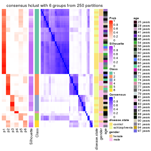
Heatmaps for the consensus matrix. It visualizes the probability of two samples to be in a same group.
consensus_heatmap(res, k = 2)
consensus_heatmap(res, k = 3)
consensus_heatmap(res, k = 4)
consensus_heatmap(res, k = 5)
consensus_heatmap(res, k = 6)
Heatmaps for the membership of samples in all partitions to see how consistent they are:
membership_heatmap(res, k = 2)
membership_heatmap(res, k = 3)
membership_heatmap(res, k = 4)
membership_heatmap(res, k = 5)
membership_heatmap(res, k = 6)
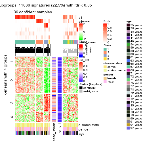
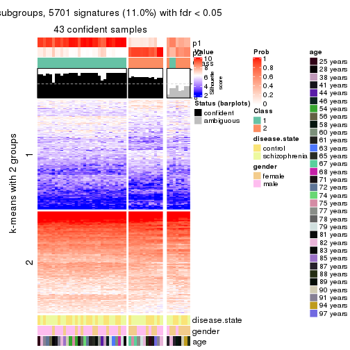
As soon as we have had the classes for columns, we can look for signatures which are significantly different between classes which can be candidate marks for certain classes. Following are the heatmaps for signatures.
Signature heatmaps where rows are scaled:
get_signatures(res, k = 2)
get_signatures(res, k = 3)
get_signatures(res, k = 4)
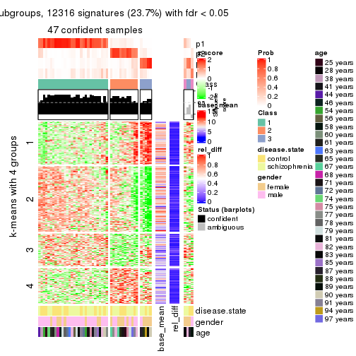
get_signatures(res, k = 5)
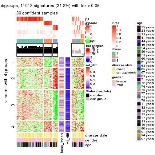
get_signatures(res, k = 6)
Signature heatmaps where rows are not scaled:
get_signatures(res, k = 2, scale_rows = FALSE)
get_signatures(res, k = 3, scale_rows = FALSE)
get_signatures(res, k = 4, scale_rows = FALSE)
get_signatures(res, k = 5, scale_rows = FALSE)
get_signatures(res, k = 6, scale_rows = FALSE)
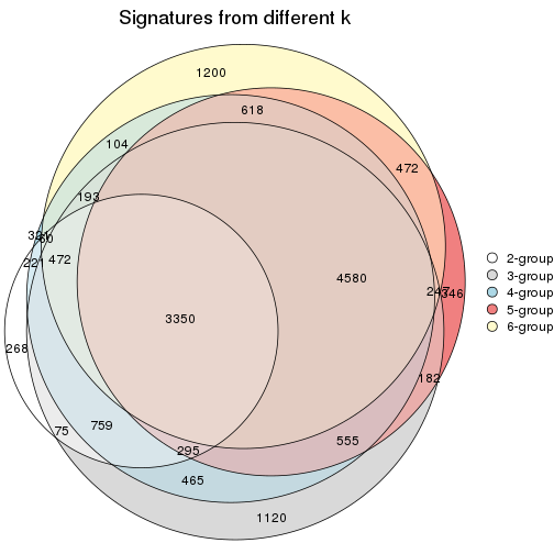
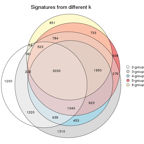
Compare the overlap of signatures from different k:
compare_signatures(res)
get_signature() returns a data frame invisibly. TO get the list of signatures, the function
call should be assigned to a variable explicitly. In following code, if plot argument is set
to FALSE, no heatmap is plotted while only the differential analysis is performed.
# code only for demonstration
tb = get_signature(res, k = ..., plot = FALSE)
An example of the output of tb is:
#>   which_row         fdr    mean_1    mean_2 scaled_mean_1 scaled_mean_2 km
#> 1        38 0.042760348  8.373488  9.131774    -0.5533452     0.5164555  1
#> 2        40 0.018707592  7.106213  8.469186    -0.6173731     0.5762149  1
#> 3        55 0.019134737 10.221463 11.207825    -0.6159697     0.5749050  1
#> 4        59 0.006059896  5.921854  7.869574    -0.6899429     0.6439467  1
#> 5        60 0.018055526  8.928898 10.211722    -0.6204761     0.5791110  1
#> 6        98 0.009384629 15.714769 14.887706     0.6635654    -0.6193277  2
...
The columns in tb are:
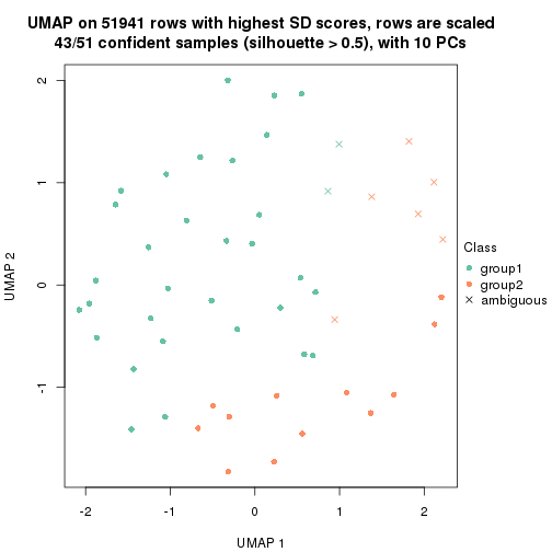
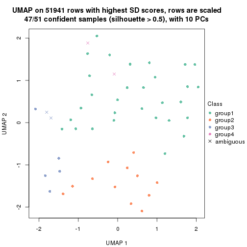
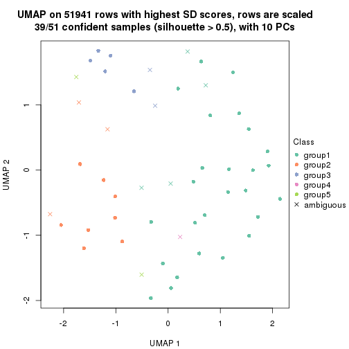
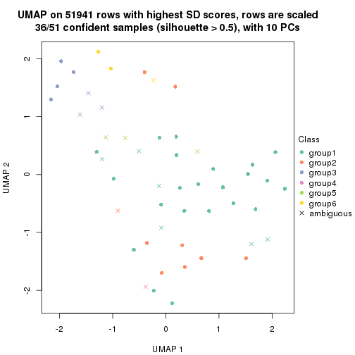
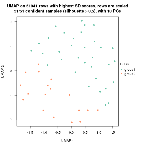
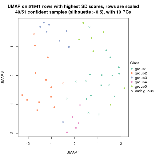
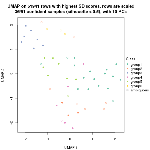
which_row: row indices corresponding to the input matrix.fdr: FDR for the differential test. mean_x: The mean value in group x.scaled_mean_x: The mean value in group x after rows are scaled.km: Row groups if k-means clustering is applied to rows.UMAP plot which shows how samples are separated.
dimension_reduction(res, k = 2, method = "UMAP")
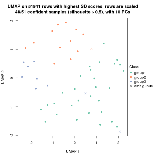
dimension_reduction(res, k = 3, method = "UMAP")

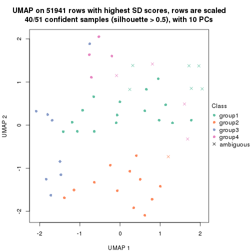
dimension_reduction(res, k = 4, method = "UMAP")
dimension_reduction(res, k = 5, method = "UMAP")
dimension_reduction(res, k = 6, method = "UMAP")
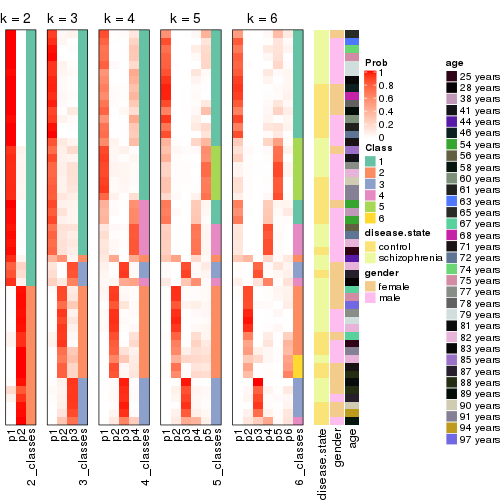
Following heatmap shows how subgroups are split when increasing k:
collect_classes(res)
Test correlation between subgroups and known annotations. If the known annotation is numeric, one-way ANOVA test is applied, and if the known annotation is discrete, chi-squared contingency table test is applied.
test_to_known_factors(res)
#>            n disease.state(p) gender(p) age(p) k
#> SD:hclust 43            1.000   0.24775  0.806 2
#> SD:hclust 48            0.983   0.00741  0.638 3
#> SD:hclust 47            0.934   0.02605  0.546 4
#> SD:hclust 39            0.790   0.06212  0.387 5
#> SD:hclust 36            0.942   0.02647  0.434 6
If matrix rows can be associated to genes, consider to use functional_enrichment(res,
...) to perform function enrichment for the signature genes. See this vignette for more detailed explanations.
The object with results only for a single top-value method and a single partition method can be extracted as:
res = res_list["SD", "kmeans"]
# you can also extract it by
# res = res_list["SD:kmeans"]
A summary of res and all the functions that can be applied to it:
res
#> A 'ConsensusPartition' object with k = 2, 3, 4, 5, 6.
#>   On a matrix with 51941 rows and 51 columns.
#>   Top rows (1000, 2000, 3000, 4000, 5000) are extracted by 'SD' method.
#>   Subgroups are detected by 'kmeans' method.
#>   Performed in total 1250 partitions by row resampling.
#>   Best k for subgroups seems to be 2.
#>
#> Following methods can be applied to this 'ConsensusPartition' object:
#>  [1] "cola_report"             "collect_classes"         "collect_plots"
#>  [4] "collect_stats"           "colnames"                "compare_signatures"
#>  [7] "consensus_heatmap"       "dimension_reduction"     "functional_enrichment"
#> [10] "get_anno_col"            "get_anno"                "get_classes"
#> [13] "get_consensus"           "get_matrix"              "get_membership"
#> [16] "get_param"               "get_signatures"          "get_stats"
#> [19] "is_best_k"               "is_stable_k"             "membership_heatmap"
#> [22] "ncol"                    "nrow"                    "plot_ecdf"
#> [25] "rownames"                "select_partition_number" "show"
#> [28] "suggest_best_k"          "test_to_known_factors"
collect_plots() function collects all the plots made from res for all k (number of partitions)
into one single page to provide an easy and fast comparison between different k.
collect_plots(res)
The plots are:
k and the heatmap of
predicted classes for each k.k.k.k.All the plots in panels can be made by individual functions and they are plotted later in this section.
select_partition_number() produces several plots showing different
statistics for choosing “optimized” k. There are following statistics:
k;k, the area increased is defined as \(A_k - A_{k-1}\).The detailed explanations of these statistics can be found in the cola vignette.
Generally speaking, lower PAC score, higher mean silhouette score or higher
concordance corresponds to better partition. Rand index and Jaccard index
measure how similar the current partition is compared to partition with k-1.
If they are too similar, we won't accept k is better than k-1.
select_partition_number(res)
The numeric values for all these statistics can be obtained by get_stats().
get_stats(res)
#>   k 1-PAC mean_silhouette concordance area_increased  Rand Jaccard
#> 2 2 0.974           0.950       0.971         0.4695 0.534   0.534
#> 3 3 0.514           0.762       0.823         0.3204 0.827   0.689
#> 4 4 0.589           0.602       0.746         0.1492 0.867   0.679
#> 5 5 0.588           0.630       0.696         0.0772 0.871   0.598
#> 6 6 0.611           0.565       0.749         0.0550 0.948   0.781
suggest_best_k() suggests the best \(k\) based on these statistics. The rules are as follows:
suggest_best_k(res)
#> [1] 2
Following shows the table of the partitions (You need to click the show/hide
code output link to see it). The membership matrix (columns with name p*)
is inferred by
clue::cl_consensus()
function with the SE method. Basically the value in the membership matrix
represents the probability to belong to a certain group. The finall class
label for an item is determined with the group with highest probability it
belongs to.
In get_classes() function, the entropy is calculated from the membership
matrix and the silhouette score is calculated from the consensus matrix.
cbind(get_classes(res, k = 2), get_membership(res, k = 2))
#>           class entropy silhouette    p1    p2
#> GSM439800     1  0.3584      0.930 0.932 0.068
#> GSM439790     1  0.0000      0.968 1.000 0.000
#> GSM439827     2  0.0938      0.972 0.012 0.988
#> GSM439811     2  0.0672      0.971 0.008 0.992
#> GSM439795     2  0.0938      0.971 0.012 0.988
#> GSM439805     1  0.7674      0.748 0.776 0.224
#> GSM439781     1  0.3733      0.931 0.928 0.072
#> GSM439807     2  0.6973      0.775 0.188 0.812
#> GSM439820     2  0.0672      0.971 0.008 0.992
#> GSM439784     1  0.2948      0.945 0.948 0.052
#> GSM439824     1  0.3114      0.936 0.944 0.056
#> GSM439794     1  0.1184      0.964 0.984 0.016
#> GSM439809     1  0.0000      0.968 1.000 0.000
#> GSM439785     1  0.0000      0.968 1.000 0.000
#> GSM439803     1  0.0672      0.966 0.992 0.008
#> GSM439778     1  0.0000      0.968 1.000 0.000
#> GSM439791     1  0.0000      0.968 1.000 0.000
#> GSM439786     1  0.3114      0.942 0.944 0.056
#> GSM439828     2  0.0938      0.969 0.012 0.988
#> GSM439806     1  0.0000      0.968 1.000 0.000
#> GSM439815     1  0.0672      0.966 0.992 0.008
#> GSM439817     2  0.0672      0.972 0.008 0.992
#> GSM439796     1  0.1184      0.964 0.984 0.016
#> GSM439798     1  0.3114      0.942 0.944 0.056
#> GSM439821     2  0.0000      0.971 0.000 1.000
#> GSM439823     2  0.0938      0.969 0.012 0.988
#> GSM439813     1  0.0000      0.968 1.000 0.000
#> GSM439801     2  0.3733      0.923 0.072 0.928
#> GSM439810     1  0.0000      0.968 1.000 0.000
#> GSM439783     1  0.0000      0.968 1.000 0.000
#> GSM439826     2  0.3431      0.930 0.064 0.936
#> GSM439812     1  0.0000      0.968 1.000 0.000
#> GSM439818     2  0.0000      0.971 0.000 1.000
#> GSM439792     1  0.0000      0.968 1.000 0.000
#> GSM439802     1  0.6623      0.823 0.828 0.172
#> GSM439825     2  0.0000      0.971 0.000 1.000
#> GSM439780     1  0.0000      0.968 1.000 0.000
#> GSM439787     2  0.0938      0.971 0.012 0.988
#> GSM439808     2  0.0672      0.971 0.008 0.992
#> GSM439804     1  0.0672      0.966 0.992 0.008
#> GSM439822     2  0.3431      0.930 0.064 0.936
#> GSM439816     1  0.0672      0.966 0.992 0.008
#> GSM439789     1  0.0672      0.966 0.992 0.008
#> GSM439799     2  0.0000      0.971 0.000 1.000
#> GSM439814     1  0.0672      0.966 0.992 0.008
#> GSM439782     1  0.0000      0.968 1.000 0.000
#> GSM439779     1  0.0000      0.968 1.000 0.000
#> GSM439793     1  0.3114      0.942 0.944 0.056
#> GSM439788     1  0.2948      0.945 0.948 0.052
#> GSM439797     1  0.3114      0.942 0.944 0.056
#> GSM439819     2  0.0000      0.971 0.000 1.000
cbind(get_classes(res, k = 3), get_membership(res, k = 3))
#>           class entropy silhouette    p1    p2    p3
#> GSM439800     3  0.8033      0.445 0.240 0.120 0.640
#> GSM439790     1  0.3669      0.842 0.896 0.040 0.064
#> GSM439827     2  0.3910      0.776 0.020 0.876 0.104
#> GSM439811     2  0.3551      0.787 0.000 0.868 0.132
#> GSM439795     3  0.2866      0.785 0.008 0.076 0.916
#> GSM439805     3  0.4164      0.718 0.144 0.008 0.848
#> GSM439781     1  0.6858      0.710 0.728 0.084 0.188
#> GSM439807     3  0.3237      0.788 0.032 0.056 0.912
#> GSM439820     2  0.5327      0.729 0.000 0.728 0.272
#> GSM439784     1  0.4469      0.820 0.864 0.076 0.060
#> GSM439824     2  0.7770      0.133 0.384 0.560 0.056
#> GSM439794     1  0.7508      0.703 0.696 0.156 0.148
#> GSM439809     1  0.2280      0.852 0.940 0.052 0.008
#> GSM439785     1  0.5094      0.834 0.832 0.112 0.056
#> GSM439803     1  0.6271      0.780 0.772 0.140 0.088
#> GSM439778     1  0.0592      0.863 0.988 0.000 0.012
#> GSM439791     1  0.0237      0.861 0.996 0.004 0.000
#> GSM439786     1  0.6488      0.742 0.756 0.084 0.160
#> GSM439828     2  0.2866      0.779 0.008 0.916 0.076
#> GSM439806     1  0.2749      0.847 0.924 0.064 0.012
#> GSM439815     1  0.2903      0.854 0.924 0.048 0.028
#> GSM439817     2  0.3784      0.790 0.004 0.864 0.132
#> GSM439796     1  0.7082      0.735 0.724 0.156 0.120
#> GSM439798     1  0.6544      0.737 0.752 0.084 0.164
#> GSM439821     2  0.5785      0.648 0.000 0.668 0.332
#> GSM439823     2  0.2866      0.779 0.008 0.916 0.076
#> GSM439813     1  0.1905      0.859 0.956 0.028 0.016
#> GSM439801     3  0.2939      0.788 0.012 0.072 0.916
#> GSM439810     1  0.1620      0.862 0.964 0.024 0.012
#> GSM439783     1  0.4384      0.833 0.868 0.068 0.064
#> GSM439826     2  0.3369      0.703 0.052 0.908 0.040
#> GSM439812     1  0.2414      0.858 0.940 0.040 0.020
#> GSM439818     2  0.4796      0.762 0.000 0.780 0.220
#> GSM439792     1  0.1267      0.862 0.972 0.024 0.004
#> GSM439802     3  0.4235      0.689 0.176 0.000 0.824
#> GSM439825     2  0.4796      0.762 0.000 0.780 0.220
#> GSM439780     1  0.3607      0.824 0.880 0.008 0.112
#> GSM439787     3  0.3043      0.782 0.008 0.084 0.908
#> GSM439808     3  0.3686      0.721 0.000 0.140 0.860
#> GSM439804     1  0.6510      0.765 0.756 0.156 0.088
#> GSM439822     2  0.2947      0.715 0.060 0.920 0.020
#> GSM439816     1  0.5696      0.788 0.796 0.148 0.056
#> GSM439789     1  0.4379      0.829 0.868 0.072 0.060
#> GSM439799     3  0.5529      0.497 0.000 0.296 0.704
#> GSM439814     1  0.3434      0.846 0.904 0.064 0.032
#> GSM439782     1  0.0592      0.863 0.988 0.000 0.012
#> GSM439779     1  0.0000      0.862 1.000 0.000 0.000
#> GSM439793     1  0.6181      0.753 0.772 0.072 0.156
#> GSM439788     1  0.5722      0.778 0.800 0.068 0.132
#> GSM439797     1  0.5998      0.811 0.788 0.128 0.084
#> GSM439819     2  0.5397      0.721 0.000 0.720 0.280
cbind(get_classes(res, k = 4), get_membership(res, k = 4))
#>           class entropy silhouette    p1    p2    p3    p4
#> GSM439800     4  0.7069     -0.273 0.036 0.048 0.440 0.476
#> GSM439790     1  0.3719      0.630 0.848 0.008 0.020 0.124
#> GSM439827     2  0.3065      0.814 0.052 0.900 0.032 0.016
#> GSM439811     2  0.2901      0.819 0.036 0.908 0.040 0.016
#> GSM439795     3  0.1114      0.907 0.004 0.016 0.972 0.008
#> GSM439805     3  0.2856      0.873 0.072 0.004 0.900 0.024
#> GSM439781     1  0.3761      0.549 0.868 0.044 0.068 0.020
#> GSM439807     3  0.1911      0.903 0.004 0.032 0.944 0.020
#> GSM439820     2  0.4141      0.785 0.004 0.820 0.144 0.032
#> GSM439784     1  0.3047      0.582 0.900 0.040 0.012 0.048
#> GSM439824     2  0.7008     -0.104 0.116 0.448 0.000 0.436
#> GSM439794     4  0.4573      0.625 0.124 0.036 0.024 0.816
#> GSM439809     1  0.4198      0.634 0.768 0.004 0.004 0.224
#> GSM439785     1  0.6212      0.351 0.592 0.056 0.004 0.348
#> GSM439803     4  0.4063      0.611 0.172 0.016 0.004 0.808
#> GSM439778     1  0.4673      0.598 0.700 0.000 0.008 0.292
#> GSM439791     1  0.4456      0.611 0.716 0.000 0.004 0.280
#> GSM439786     1  0.3824      0.538 0.868 0.056 0.048 0.028
#> GSM439828     2  0.2319      0.822 0.028 0.932 0.016 0.024
#> GSM439806     1  0.4489      0.635 0.780 0.024 0.004 0.192
#> GSM439815     1  0.5257      0.331 0.548 0.000 0.008 0.444
#> GSM439817     2  0.2188      0.826 0.020 0.936 0.032 0.012
#> GSM439796     4  0.4412      0.627 0.128 0.036 0.016 0.820
#> GSM439798     1  0.3984      0.531 0.860 0.060 0.052 0.028
#> GSM439821     2  0.6370      0.602 0.000 0.620 0.280 0.100
#> GSM439823     2  0.2616      0.819 0.028 0.920 0.016 0.036
#> GSM439813     1  0.5039      0.429 0.592 0.000 0.004 0.404
#> GSM439801     3  0.2170      0.902 0.008 0.028 0.936 0.028
#> GSM439810     1  0.5522      0.545 0.648 0.016 0.012 0.324
#> GSM439783     4  0.5811      0.137 0.408 0.020 0.008 0.564
#> GSM439826     2  0.3123      0.789 0.000 0.844 0.000 0.156
#> GSM439812     1  0.5852      0.432 0.588 0.020 0.012 0.380
#> GSM439818     2  0.3706      0.812 0.000 0.848 0.040 0.112
#> GSM439792     1  0.5278      0.592 0.688 0.020 0.008 0.284
#> GSM439802     3  0.2669      0.882 0.052 0.004 0.912 0.032
#> GSM439825     2  0.4153      0.804 0.000 0.820 0.048 0.132
#> GSM439780     1  0.4959      0.620 0.768 0.008 0.044 0.180
#> GSM439787     3  0.0927      0.905 0.000 0.016 0.976 0.008
#> GSM439808     3  0.2089      0.888 0.000 0.048 0.932 0.020
#> GSM439804     4  0.4182      0.627 0.140 0.036 0.004 0.820
#> GSM439822     2  0.3893      0.781 0.000 0.796 0.008 0.196
#> GSM439816     4  0.5587      0.282 0.372 0.028 0.000 0.600
#> GSM439789     4  0.4843      0.212 0.396 0.000 0.000 0.604
#> GSM439799     3  0.6626      0.639 0.004 0.116 0.620 0.260
#> GSM439814     1  0.5126      0.310 0.552 0.000 0.004 0.444
#> GSM439782     1  0.4673      0.597 0.700 0.000 0.008 0.292
#> GSM439779     1  0.4511      0.615 0.724 0.000 0.008 0.268
#> GSM439793     1  0.3285      0.558 0.892 0.032 0.052 0.024
#> GSM439788     1  0.2807      0.565 0.912 0.032 0.040 0.016
#> GSM439797     1  0.5353      0.388 0.752 0.072 0.008 0.168
#> GSM439819     2  0.4966      0.760 0.000 0.768 0.156 0.076
cbind(get_classes(res, k = 5), get_membership(res, k = 5))
#>           class entropy silhouette    p1    p2    p3    p4    p5
#> GSM439800     4  0.6341     0.2468 0.108 0.004 0.296 0.572 0.020
#> GSM439790     1  0.5242    -0.0585 0.556 0.000 0.004 0.040 0.400
#> GSM439827     2  0.1960     0.7604 0.004 0.936 0.012 0.020 0.028
#> GSM439811     2  0.2064     0.7595 0.004 0.932 0.016 0.020 0.028
#> GSM439795     3  0.0727     0.8216 0.000 0.004 0.980 0.012 0.004
#> GSM439805     3  0.3444     0.7709 0.024 0.000 0.848 0.024 0.104
#> GSM439781     5  0.6105     0.7851 0.324 0.044 0.020 0.024 0.588
#> GSM439807     3  0.3792     0.8053 0.000 0.068 0.840 0.056 0.036
#> GSM439820     2  0.4246     0.7159 0.000 0.812 0.060 0.084 0.044
#> GSM439784     5  0.4814     0.6780 0.412 0.016 0.004 0.000 0.568
#> GSM439824     2  0.7046     0.0994 0.300 0.476 0.000 0.196 0.028
#> GSM439794     4  0.4896     0.8365 0.248 0.004 0.004 0.696 0.048
#> GSM439809     1  0.2719     0.5993 0.852 0.004 0.000 0.000 0.144
#> GSM439785     1  0.6951    -0.0277 0.396 0.012 0.000 0.216 0.376
#> GSM439803     4  0.4969     0.8137 0.264 0.004 0.000 0.676 0.056
#> GSM439778     1  0.4836     0.5720 0.716 0.000 0.000 0.096 0.188
#> GSM439791     1  0.3897     0.5818 0.768 0.000 0.000 0.028 0.204
#> GSM439786     5  0.4456     0.8379 0.228 0.016 0.016 0.004 0.736
#> GSM439828     2  0.1741     0.7631 0.000 0.936 0.000 0.024 0.040
#> GSM439806     1  0.3487     0.4928 0.780 0.008 0.000 0.000 0.212
#> GSM439815     1  0.3193     0.6252 0.840 0.000 0.000 0.132 0.028
#> GSM439817     2  0.1278     0.7632 0.000 0.960 0.004 0.016 0.020
#> GSM439796     4  0.4768     0.8360 0.252 0.004 0.000 0.696 0.048
#> GSM439798     5  0.4301     0.8395 0.228 0.016 0.016 0.000 0.740
#> GSM439821     2  0.8250     0.3927 0.000 0.404 0.216 0.200 0.180
#> GSM439823     2  0.2149     0.7597 0.000 0.916 0.000 0.036 0.048
#> GSM439813     1  0.1914     0.6643 0.924 0.000 0.000 0.060 0.016
#> GSM439801     3  0.2993     0.8013 0.000 0.048 0.884 0.044 0.024
#> GSM439810     1  0.1059     0.6625 0.968 0.000 0.004 0.020 0.008
#> GSM439783     1  0.4975     0.4261 0.668 0.000 0.004 0.276 0.052
#> GSM439826     2  0.4376     0.7222 0.012 0.768 0.000 0.172 0.048
#> GSM439812     1  0.1041     0.6638 0.964 0.000 0.004 0.032 0.000
#> GSM439818     2  0.5578     0.7277 0.012 0.708 0.016 0.140 0.124
#> GSM439792     1  0.2982     0.6430 0.860 0.000 0.004 0.020 0.116
#> GSM439802     3  0.2875     0.7973 0.020 0.000 0.888 0.032 0.060
#> GSM439825     2  0.6587     0.6729 0.012 0.592 0.016 0.200 0.180
#> GSM439780     1  0.5071     0.2467 0.628 0.000 0.008 0.036 0.328
#> GSM439787     3  0.1934     0.8217 0.000 0.008 0.932 0.040 0.020
#> GSM439808     3  0.4376     0.7866 0.000 0.072 0.804 0.080 0.044
#> GSM439804     4  0.4743     0.8358 0.248 0.004 0.000 0.700 0.048
#> GSM439822     2  0.5499     0.6941 0.004 0.652 0.000 0.232 0.112
#> GSM439816     1  0.5378     0.2909 0.648 0.024 0.000 0.284 0.044
#> GSM439789     1  0.4339     0.3698 0.684 0.000 0.000 0.296 0.020
#> GSM439799     3  0.7257     0.2974 0.000 0.104 0.428 0.388 0.080
#> GSM439814     1  0.1892     0.6614 0.916 0.000 0.000 0.080 0.004
#> GSM439782     1  0.5122     0.5524 0.688 0.000 0.000 0.112 0.200
#> GSM439779     1  0.2719     0.6346 0.852 0.000 0.000 0.004 0.144
#> GSM439793     5  0.4854     0.8400 0.312 0.016 0.012 0.004 0.656
#> GSM439788     5  0.4537     0.8365 0.312 0.012 0.004 0.004 0.668
#> GSM439797     5  0.5262     0.7800 0.196 0.028 0.000 0.068 0.708
#> GSM439819     2  0.6781     0.6086 0.000 0.604 0.084 0.168 0.144
cbind(get_classes(res, k = 6), get_membership(res, k = 6))
#>           class entropy silhouette    p1    p2    p3    p4    p5    p6
#> GSM439800     4  0.6023     0.5133 0.068 0.000 0.148 0.628 0.008 0.148
#> GSM439790     1  0.6166     0.2240 0.508 0.008 0.000 0.036 0.344 0.104
#> GSM439827     2  0.3093     0.4941 0.012 0.864 0.000 0.012 0.048 0.064
#> GSM439811     2  0.3141     0.4907 0.012 0.860 0.000 0.012 0.044 0.072
#> GSM439795     3  0.0000     0.8203 0.000 0.000 1.000 0.000 0.000 0.000
#> GSM439805     3  0.4631     0.7154 0.016 0.004 0.756 0.024 0.144 0.056
#> GSM439781     5  0.5153     0.7468 0.164 0.028 0.004 0.024 0.716 0.064
#> GSM439807     3  0.4356     0.7827 0.000 0.036 0.780 0.060 0.012 0.112
#> GSM439820     2  0.3243     0.4110 0.000 0.848 0.032 0.024 0.004 0.092
#> GSM439784     5  0.3876     0.7243 0.244 0.016 0.000 0.012 0.728 0.000
#> GSM439824     2  0.7812     0.0346 0.276 0.372 0.000 0.208 0.028 0.116
#> GSM439794     4  0.2834     0.7793 0.128 0.000 0.000 0.848 0.016 0.008
#> GSM439809     1  0.3624     0.6905 0.808 0.008 0.000 0.012 0.140 0.032
#> GSM439785     5  0.6274     0.3234 0.264 0.008 0.000 0.220 0.496 0.012
#> GSM439803     4  0.3275     0.7549 0.144 0.000 0.000 0.816 0.036 0.004
#> GSM439778     1  0.5386     0.6316 0.676 0.000 0.000 0.112 0.152 0.060
#> GSM439791     1  0.3601     0.6951 0.792 0.000 0.000 0.040 0.160 0.008
#> GSM439786     5  0.3121     0.7732 0.060 0.016 0.004 0.004 0.864 0.052
#> GSM439828     2  0.1082     0.5111 0.000 0.956 0.000 0.004 0.040 0.000
#> GSM439806     1  0.3780     0.6222 0.760 0.016 0.000 0.000 0.204 0.020
#> GSM439815     1  0.3757     0.6988 0.804 0.000 0.000 0.120 0.024 0.052
#> GSM439817     2  0.0551     0.5133 0.000 0.984 0.000 0.004 0.008 0.004
#> GSM439796     4  0.2809     0.7791 0.128 0.000 0.000 0.848 0.020 0.004
#> GSM439798     5  0.3060     0.7727 0.056 0.016 0.004 0.004 0.868 0.052
#> GSM439821     6  0.6839     0.3037 0.000 0.272 0.200 0.040 0.016 0.472
#> GSM439823     2  0.1536     0.5073 0.000 0.940 0.000 0.016 0.040 0.004
#> GSM439813     1  0.2340     0.7173 0.896 0.000 0.000 0.056 0.004 0.044
#> GSM439801     3  0.3154     0.7737 0.000 0.048 0.868 0.020 0.024 0.040
#> GSM439810     1  0.1924     0.7218 0.920 0.000 0.000 0.004 0.028 0.048
#> GSM439783     1  0.5183     0.5134 0.640 0.000 0.000 0.264 0.048 0.048
#> GSM439826     2  0.4991     0.1467 0.000 0.648 0.000 0.100 0.008 0.244
#> GSM439812     1  0.2282     0.7153 0.900 0.000 0.000 0.012 0.020 0.068
#> GSM439818     6  0.4488     0.2800 0.000 0.468 0.008 0.016 0.000 0.508
#> GSM439792     1  0.3621     0.6853 0.808 0.000 0.000 0.024 0.132 0.036
#> GSM439802     3  0.3574     0.7876 0.016 0.004 0.840 0.016 0.044 0.080
#> GSM439825     6  0.4387     0.4729 0.000 0.344 0.008 0.016 0.004 0.628
#> GSM439780     1  0.5398     0.4976 0.640 0.000 0.000 0.040 0.232 0.088
#> GSM439787     3  0.1951     0.8151 0.000 0.000 0.916 0.020 0.004 0.060
#> GSM439808     3  0.5145     0.7411 0.000 0.068 0.724 0.064 0.016 0.128
#> GSM439804     4  0.2920     0.7810 0.128 0.000 0.000 0.844 0.020 0.008
#> GSM439822     2  0.5693    -0.2764 0.000 0.468 0.000 0.140 0.004 0.388
#> GSM439816     1  0.5985     0.3498 0.568 0.012 0.000 0.284 0.028 0.108
#> GSM439789     1  0.4253     0.5001 0.668 0.000 0.000 0.300 0.012 0.020
#> GSM439799     4  0.7454     0.1657 0.000 0.128 0.256 0.452 0.024 0.140
#> GSM439814     1  0.2680     0.7149 0.880 0.000 0.000 0.060 0.012 0.048
#> GSM439782     1  0.5663     0.6112 0.648 0.000 0.000 0.136 0.152 0.064
#> GSM439779     1  0.2760     0.7147 0.856 0.000 0.000 0.024 0.116 0.004
#> GSM439793     5  0.3317     0.7964 0.168 0.016 0.000 0.012 0.804 0.000
#> GSM439788     5  0.3324     0.7962 0.164 0.016 0.000 0.008 0.808 0.004
#> GSM439797     5  0.3348     0.7962 0.084 0.016 0.000 0.036 0.848 0.016
#> GSM439819     2  0.6115    -0.3197 0.000 0.508 0.080 0.040 0.012 0.360
Heatmaps for the consensus matrix. It visualizes the probability of two samples to be in a same group.
consensus_heatmap(res, k = 2)
consensus_heatmap(res, k = 3)
consensus_heatmap(res, k = 4)
consensus_heatmap(res, k = 5)
consensus_heatmap(res, k = 6)
Heatmaps for the membership of samples in all partitions to see how consistent they are:
membership_heatmap(res, k = 2)
membership_heatmap(res, k = 3)
membership_heatmap(res, k = 4)
membership_heatmap(res, k = 5)
membership_heatmap(res, k = 6)
As soon as we have had the classes for columns, we can look for signatures which are significantly different between classes which can be candidate marks for certain classes. Following are the heatmaps for signatures.
Signature heatmaps where rows are scaled:
get_signatures(res, k = 2)
get_signatures(res, k = 3)
get_signatures(res, k = 4)
get_signatures(res, k = 5)
get_signatures(res, k = 6)
Signature heatmaps where rows are not scaled:
get_signatures(res, k = 2, scale_rows = FALSE)
get_signatures(res, k = 3, scale_rows = FALSE)
get_signatures(res, k = 4, scale_rows = FALSE)
get_signatures(res, k = 5, scale_rows = FALSE)
get_signatures(res, k = 6, scale_rows = FALSE)
Compare the overlap of signatures from different k:
compare_signatures(res)
get_signature() returns a data frame invisibly. TO get the list of signatures, the function
call should be assigned to a variable explicitly. In following code, if plot argument is set
to FALSE, no heatmap is plotted while only the differential analysis is performed.
# code only for demonstration
tb = get_signature(res, k = ..., plot = FALSE)
An example of the output of tb is:
#>   which_row         fdr    mean_1    mean_2 scaled_mean_1 scaled_mean_2 km
#> 1        38 0.042760348  8.373488  9.131774    -0.5533452     0.5164555  1
#> 2        40 0.018707592  7.106213  8.469186    -0.6173731     0.5762149  1
#> 3        55 0.019134737 10.221463 11.207825    -0.6159697     0.5749050  1
#> 4        59 0.006059896  5.921854  7.869574    -0.6899429     0.6439467  1
#> 5        60 0.018055526  8.928898 10.211722    -0.6204761     0.5791110  1
#> 6        98 0.009384629 15.714769 14.887706     0.6635654    -0.6193277  2
...
The columns in tb are:
which_row: row indices corresponding to the input matrix.fdr: FDR for the differential test. mean_x: The mean value in group x.scaled_mean_x: The mean value in group x after rows are scaled.km: Row groups if k-means clustering is applied to rows.UMAP plot which shows how samples are separated.
dimension_reduction(res, k = 2, method = "UMAP")
dimension_reduction(res, k = 3, method = "UMAP")
dimension_reduction(res, k = 4, method = "UMAP")
dimension_reduction(res, k = 5, method = "UMAP")
dimension_reduction(res, k = 6, method = "UMAP")
Following heatmap shows how subgroups are split when increasing k:
collect_classes(res)
Test correlation between subgroups and known annotations. If the known annotation is numeric, one-way ANOVA test is applied, and if the known annotation is discrete, chi-squared contingency table test is applied.
test_to_known_factors(res)
#>            n disease.state(p) gender(p) age(p) k
#> SD:kmeans 51            1.000   0.14290  0.729 2
#> SD:kmeans 48            0.915   0.00796  0.580 3
#> SD:kmeans 40            0.873   0.05707  0.658 4
#> SD:kmeans 40            0.898   0.01460  0.510 5
#> SD:kmeans 36            0.343   0.01867  0.551 6
If matrix rows can be associated to genes, consider to use functional_enrichment(res,
...) to perform function enrichment for the signature genes. See this vignette for more detailed explanations.
The object with results only for a single top-value method and a single partition method can be extracted as:
res = res_list["SD", "skmeans"]
# you can also extract it by
# res = res_list["SD:skmeans"]
A summary of res and all the functions that can be applied to it:
res
#> A 'ConsensusPartition' object with k = 2, 3, 4, 5, 6.
#>   On a matrix with 51941 rows and 51 columns.
#>   Top rows (1000, 2000, 3000, 4000, 5000) are extracted by 'SD' method.
#>   Subgroups are detected by 'skmeans' method.
#>   Performed in total 1250 partitions by row resampling.
#>   Best k for subgroups seems to be 2.
#>
#> Following methods can be applied to this 'ConsensusPartition' object:
#>  [1] "cola_report"             "collect_classes"         "collect_plots"
#>  [4] "collect_stats"           "colnames"                "compare_signatures"
#>  [7] "consensus_heatmap"       "dimension_reduction"     "functional_enrichment"
#> [10] "get_anno_col"            "get_anno"                "get_classes"
#> [13] "get_consensus"           "get_matrix"              "get_membership"
#> [16] "get_param"               "get_signatures"          "get_stats"
#> [19] "is_best_k"               "is_stable_k"             "membership_heatmap"
#> [22] "ncol"                    "nrow"                    "plot_ecdf"
#> [25] "rownames"                "select_partition_number" "show"
#> [28] "suggest_best_k"          "test_to_known_factors"
collect_plots() function collects all the plots made from res for all k (number of partitions)
into one single page to provide an easy and fast comparison between different k.
collect_plots(res)
The plots are:
k and the heatmap of
predicted classes for each k.k.k.k.All the plots in panels can be made by individual functions and they are plotted later in this section.
select_partition_number() produces several plots showing different
statistics for choosing “optimized” k. There are following statistics:
k;k, the area increased is defined as \(A_k - A_{k-1}\).The detailed explanations of these statistics can be found in the cola vignette.
Generally speaking, lower PAC score, higher mean silhouette score or higher
concordance corresponds to better partition. Rand index and Jaccard index
measure how similar the current partition is compared to partition with k-1.
If they are too similar, we won't accept k is better than k-1.
select_partition_number(res)
The numeric values for all these statistics can be obtained by get_stats().
get_stats(res)
#>   k 1-PAC mean_silhouette concordance area_increased  Rand Jaccard
#> 2 2 0.566           0.789       0.911         0.5041 0.500   0.500
#> 3 3 0.286           0.473       0.701         0.3289 0.740   0.528
#> 4 4 0.302           0.351       0.583         0.1243 0.843   0.593
#> 5 5 0.388           0.406       0.576         0.0639 0.910   0.688
#> 6 6 0.475           0.365       0.560         0.0421 0.974   0.886
suggest_best_k() suggests the best \(k\) based on these statistics. The rules are as follows:
suggest_best_k(res)
#> [1] 2
Following shows the table of the partitions (You need to click the show/hide
code output link to see it). The membership matrix (columns with name p*)
is inferred by
clue::cl_consensus()
function with the SE method. Basically the value in the membership matrix
represents the probability to belong to a certain group. The finall class
label for an item is determined with the group with highest probability it
belongs to.
In get_classes() function, the entropy is calculated from the membership
matrix and the silhouette score is calculated from the consensus matrix.
cbind(get_classes(res, k = 2), get_membership(res, k = 2))
#>           class entropy silhouette    p1    p2
#> GSM439800     2  0.8499     0.6234 0.276 0.724
#> GSM439790     1  0.2236     0.8784 0.964 0.036
#> GSM439827     2  0.0000     0.9065 0.000 1.000
#> GSM439811     2  0.0000     0.9065 0.000 1.000
#> GSM439795     2  0.0376     0.9049 0.004 0.996
#> GSM439805     2  0.8267     0.6012 0.260 0.740
#> GSM439781     1  0.9881     0.2900 0.564 0.436
#> GSM439807     2  0.3114     0.8693 0.056 0.944
#> GSM439820     2  0.0000     0.9065 0.000 1.000
#> GSM439784     1  0.5519     0.8291 0.872 0.128
#> GSM439824     2  0.9998     0.0140 0.492 0.508
#> GSM439794     2  0.9983     0.0892 0.476 0.524
#> GSM439809     1  0.0000     0.8886 1.000 0.000
#> GSM439785     1  0.5178     0.8253 0.884 0.116
#> GSM439803     1  0.6148     0.7853 0.848 0.152
#> GSM439778     1  0.0000     0.8886 1.000 0.000
#> GSM439791     1  0.0000     0.8886 1.000 0.000
#> GSM439786     1  0.5178     0.8317 0.884 0.116
#> GSM439828     2  0.0000     0.9065 0.000 1.000
#> GSM439806     1  0.0000     0.8886 1.000 0.000
#> GSM439815     1  0.0938     0.8860 0.988 0.012
#> GSM439817     2  0.0000     0.9065 0.000 1.000
#> GSM439796     1  0.9998    -0.0252 0.508 0.492
#> GSM439798     1  0.6438     0.7906 0.836 0.164
#> GSM439821     2  0.0000     0.9065 0.000 1.000
#> GSM439823     2  0.0376     0.9049 0.004 0.996
#> GSM439813     1  0.0000     0.8886 1.000 0.000
#> GSM439801     2  0.1414     0.8963 0.020 0.980
#> GSM439810     1  0.0000     0.8886 1.000 0.000
#> GSM439783     1  0.0000     0.8886 1.000 0.000
#> GSM439826     2  0.4022     0.8496 0.080 0.920
#> GSM439812     1  0.0000     0.8886 1.000 0.000
#> GSM439818     2  0.0000     0.9065 0.000 1.000
#> GSM439792     1  0.0000     0.8886 1.000 0.000
#> GSM439802     1  0.9881     0.2702 0.564 0.436
#> GSM439825     2  0.0000     0.9065 0.000 1.000
#> GSM439780     1  0.0000     0.8886 1.000 0.000
#> GSM439787     2  0.0376     0.9048 0.004 0.996
#> GSM439808     2  0.0000     0.9065 0.000 1.000
#> GSM439804     1  0.7453     0.7079 0.788 0.212
#> GSM439822     2  0.3733     0.8564 0.072 0.928
#> GSM439816     1  0.3431     0.8632 0.936 0.064
#> GSM439789     1  0.0000     0.8886 1.000 0.000
#> GSM439799     2  0.0000     0.9065 0.000 1.000
#> GSM439814     1  0.0000     0.8886 1.000 0.000
#> GSM439782     1  0.0000     0.8886 1.000 0.000
#> GSM439779     1  0.0000     0.8886 1.000 0.000
#> GSM439793     1  0.5629     0.8231 0.868 0.132
#> GSM439788     1  0.3274     0.8650 0.940 0.060
#> GSM439797     1  0.8016     0.7148 0.756 0.244
#> GSM439819     2  0.0000     0.9065 0.000 1.000
cbind(get_classes(res, k = 3), get_membership(res, k = 3))
#>           class entropy silhouette    p1    p2    p3
#> GSM439800     2   0.993    -0.0528 0.288 0.388 0.324
#> GSM439790     1   0.739     0.1162 0.508 0.460 0.032
#> GSM439827     3   0.492     0.7443 0.164 0.020 0.816
#> GSM439811     3   0.378     0.7855 0.132 0.004 0.864
#> GSM439795     3   0.663     0.5077 0.392 0.012 0.596
#> GSM439805     1   0.871    -0.0845 0.484 0.108 0.408
#> GSM439781     1   0.835     0.4814 0.628 0.176 0.196
#> GSM439807     3   0.764     0.4592 0.372 0.052 0.576
#> GSM439820     3   0.295     0.7846 0.088 0.004 0.908
#> GSM439784     1   0.835     0.4176 0.576 0.320 0.104
#> GSM439824     2   0.908     0.1514 0.140 0.468 0.392
#> GSM439794     2   0.963     0.1840 0.288 0.468 0.244
#> GSM439809     2   0.625     0.2384 0.376 0.620 0.004
#> GSM439785     2   0.854     0.1653 0.404 0.500 0.096
#> GSM439803     2   0.786     0.3718 0.284 0.628 0.088
#> GSM439778     2   0.514     0.4581 0.252 0.748 0.000
#> GSM439791     2   0.536     0.4153 0.276 0.724 0.000
#> GSM439786     1   0.550     0.5081 0.744 0.248 0.008
#> GSM439828     3   0.462     0.7568 0.136 0.024 0.840
#> GSM439806     2   0.660     0.0752 0.428 0.564 0.008
#> GSM439815     2   0.690     0.3925 0.268 0.684 0.048
#> GSM439817     3   0.369     0.7811 0.100 0.016 0.884
#> GSM439796     2   0.911     0.2796 0.212 0.548 0.240
#> GSM439798     1   0.551     0.5427 0.784 0.188 0.028
#> GSM439821     3   0.226     0.7910 0.068 0.000 0.932
#> GSM439823     3   0.516     0.7410 0.140 0.040 0.820
#> GSM439813     2   0.435     0.4862 0.184 0.816 0.000
#> GSM439801     3   0.706     0.4756 0.404 0.024 0.572
#> GSM439810     2   0.424     0.4990 0.176 0.824 0.000
#> GSM439783     2   0.566     0.4784 0.200 0.772 0.028
#> GSM439826     3   0.671     0.6107 0.072 0.196 0.732
#> GSM439812     2   0.478     0.4960 0.164 0.820 0.016
#> GSM439818     3   0.203     0.7916 0.032 0.016 0.952
#> GSM439792     2   0.558     0.4297 0.256 0.736 0.008
#> GSM439802     1   0.834     0.4120 0.624 0.152 0.224
#> GSM439825     3   0.231     0.7901 0.032 0.024 0.944
#> GSM439780     1   0.730     0.0926 0.488 0.484 0.028
#> GSM439787     3   0.568     0.6206 0.316 0.000 0.684
#> GSM439808     3   0.473     0.7324 0.196 0.004 0.800
#> GSM439804     2   0.790     0.3916 0.192 0.664 0.144
#> GSM439822     3   0.560     0.6863 0.052 0.148 0.800
#> GSM439816     2   0.659     0.4479 0.092 0.752 0.156
#> GSM439789     2   0.226     0.5229 0.068 0.932 0.000
#> GSM439799     3   0.475     0.7699 0.184 0.008 0.808
#> GSM439814     2   0.254     0.5223 0.080 0.920 0.000
#> GSM439782     2   0.550     0.4058 0.292 0.708 0.000
#> GSM439779     2   0.529     0.4073 0.268 0.732 0.000
#> GSM439793     1   0.670     0.5143 0.684 0.280 0.036
#> GSM439788     1   0.580     0.4643 0.712 0.280 0.008
#> GSM439797     1   0.868     0.2657 0.572 0.288 0.140
#> GSM439819     3   0.175     0.7924 0.048 0.000 0.952
cbind(get_classes(res, k = 4), get_membership(res, k = 4))
#>           class entropy silhouette    p1    p2    p3    p4
#> GSM439800     3   0.832    0.27347 0.236 0.132 0.544 0.088
#> GSM439790     4   0.770   -0.02140 0.392 0.008 0.168 0.432
#> GSM439827     2   0.537    0.58913 0.016 0.768 0.084 0.132
#> GSM439811     2   0.523    0.59833 0.016 0.780 0.100 0.104
#> GSM439795     3   0.811    0.05028 0.016 0.376 0.404 0.204
#> GSM439805     3   0.948    0.10302 0.144 0.172 0.360 0.324
#> GSM439781     4   0.758    0.40164 0.100 0.092 0.180 0.628
#> GSM439807     3   0.877    0.14855 0.064 0.324 0.428 0.184
#> GSM439820     2   0.366    0.61154 0.008 0.864 0.088 0.040
#> GSM439784     4   0.827    0.38821 0.248 0.116 0.092 0.544
#> GSM439824     2   0.896   -0.01015 0.356 0.372 0.204 0.068
#> GSM439794     3   0.883    0.05936 0.332 0.136 0.436 0.096
#> GSM439809     1   0.663    0.30545 0.544 0.016 0.052 0.388
#> GSM439785     1   0.933    0.03360 0.324 0.084 0.284 0.308
#> GSM439803     1   0.797    0.08679 0.424 0.028 0.408 0.140
#> GSM439778     1   0.618    0.41691 0.624 0.000 0.080 0.296
#> GSM439791     1   0.676    0.39838 0.576 0.000 0.124 0.300
#> GSM439786     4   0.530    0.51772 0.152 0.012 0.072 0.764
#> GSM439828     2   0.475    0.61904 0.008 0.804 0.100 0.088
#> GSM439806     1   0.670    0.29157 0.540 0.008 0.072 0.380
#> GSM439815     1   0.816    0.36385 0.548 0.056 0.188 0.208
#> GSM439817     2   0.386    0.63577 0.004 0.848 0.104 0.044
#> GSM439796     3   0.766    0.09921 0.296 0.112 0.552 0.040
#> GSM439798     4   0.459    0.57686 0.084 0.032 0.056 0.828
#> GSM439821     2   0.376    0.59058 0.000 0.832 0.144 0.024
#> GSM439823     2   0.521    0.60426 0.012 0.776 0.124 0.088
#> GSM439813     1   0.525    0.50835 0.744 0.000 0.080 0.176
#> GSM439801     2   0.827   -0.13419 0.020 0.388 0.372 0.220
#> GSM439810     1   0.521    0.49824 0.748 0.000 0.080 0.172
#> GSM439783     1   0.745    0.41396 0.572 0.020 0.256 0.152
#> GSM439826     2   0.640    0.49114 0.096 0.664 0.228 0.012
#> GSM439812     1   0.623    0.47822 0.704 0.016 0.140 0.140
#> GSM439818     2   0.372    0.62206 0.000 0.820 0.168 0.012
#> GSM439792     1   0.690    0.39153 0.604 0.008 0.128 0.260
#> GSM439802     3   0.866    0.04761 0.116 0.092 0.428 0.364
#> GSM439825     2   0.424    0.61806 0.012 0.808 0.164 0.016
#> GSM439780     1   0.781    0.01858 0.436 0.012 0.168 0.384
#> GSM439787     2   0.799   -0.09567 0.008 0.416 0.348 0.228
#> GSM439808     2   0.665    0.29512 0.000 0.584 0.304 0.112
#> GSM439804     3   0.864    0.00753 0.324 0.104 0.464 0.108
#> GSM439822     2   0.561    0.53958 0.068 0.712 0.216 0.004
#> GSM439816     1   0.856    0.17777 0.496 0.192 0.248 0.064
#> GSM439789     1   0.495    0.50782 0.772 0.000 0.144 0.084
#> GSM439799     2   0.634    0.31160 0.000 0.552 0.380 0.068
#> GSM439814     1   0.502    0.52386 0.780 0.004 0.100 0.116
#> GSM439782     1   0.647    0.42758 0.612 0.000 0.108 0.280
#> GSM439779     1   0.540    0.43023 0.644 0.000 0.028 0.328
#> GSM439793     4   0.614    0.54552 0.140 0.036 0.096 0.728
#> GSM439788     4   0.521    0.52716 0.156 0.004 0.080 0.760
#> GSM439797     4   0.852    0.36869 0.116 0.152 0.188 0.544
#> GSM439819     2   0.260    0.62397 0.000 0.908 0.068 0.024
cbind(get_classes(res, k = 5), get_membership(res, k = 5))
#>           class entropy silhouette    p1    p2    p3    p4    p5
#> GSM439800     4   0.889     0.2438 0.144 0.144 0.292 0.372 0.048
#> GSM439790     5   0.894    -0.0605 0.280 0.024 0.200 0.176 0.320
#> GSM439827     2   0.490     0.5837 0.012 0.776 0.096 0.028 0.088
#> GSM439811     2   0.561     0.5440 0.000 0.700 0.172 0.056 0.072
#> GSM439795     3   0.471     0.6140 0.004 0.124 0.780 0.048 0.044
#> GSM439805     3   0.819     0.3138 0.064 0.072 0.508 0.148 0.208
#> GSM439781     5   0.885     0.2904 0.100 0.104 0.260 0.112 0.424
#> GSM439807     3   0.684     0.5574 0.076 0.168 0.644 0.060 0.052
#> GSM439820     2   0.634     0.3994 0.016 0.612 0.272 0.044 0.056
#> GSM439784     5   0.822     0.3362 0.216 0.080 0.128 0.068 0.508
#> GSM439824     2   0.868    -0.0381 0.228 0.412 0.040 0.216 0.104
#> GSM439794     4   0.794     0.5456 0.108 0.124 0.164 0.552 0.052
#> GSM439809     1   0.670     0.4366 0.584 0.012 0.028 0.132 0.244
#> GSM439785     5   0.882     0.1063 0.148 0.120 0.052 0.296 0.384
#> GSM439803     4   0.709     0.4158 0.140 0.048 0.072 0.632 0.108
#> GSM439778     1   0.759     0.3459 0.492 0.004 0.072 0.208 0.224
#> GSM439791     1   0.731     0.3735 0.540 0.012 0.052 0.168 0.228
#> GSM439786     5   0.604     0.4790 0.104 0.028 0.064 0.092 0.712
#> GSM439828     2   0.418     0.6060 0.008 0.820 0.048 0.028 0.096
#> GSM439806     1   0.747     0.2553 0.500 0.032 0.048 0.104 0.316
#> GSM439815     1   0.772     0.3309 0.540 0.028 0.084 0.208 0.140
#> GSM439817     2   0.493     0.5919 0.012 0.780 0.096 0.048 0.064
#> GSM439796     4   0.635     0.5814 0.112 0.112 0.068 0.684 0.024
#> GSM439798     5   0.558     0.5051 0.056 0.016 0.172 0.040 0.716
#> GSM439821     2   0.517     0.3722 0.000 0.616 0.332 0.048 0.004
#> GSM439823     2   0.622     0.5418 0.016 0.688 0.068 0.120 0.108
#> GSM439813     1   0.559     0.5161 0.720 0.008 0.040 0.136 0.096
#> GSM439801     3   0.670     0.5527 0.008 0.148 0.636 0.092 0.116
#> GSM439810     1   0.625     0.4954 0.696 0.032 0.060 0.092 0.120
#> GSM439783     1   0.758     0.3719 0.508 0.024 0.068 0.288 0.112
#> GSM439826     2   0.541     0.5315 0.048 0.720 0.032 0.184 0.016
#> GSM439812     1   0.601     0.5031 0.712 0.032 0.068 0.128 0.060
#> GSM439818     2   0.503     0.5535 0.008 0.720 0.192 0.076 0.004
#> GSM439792     1   0.694     0.4163 0.592 0.008 0.072 0.116 0.212
#> GSM439802     3   0.677     0.3747 0.064 0.032 0.648 0.104 0.152
#> GSM439825     2   0.540     0.5712 0.020 0.736 0.132 0.092 0.020
#> GSM439780     1   0.827     0.1206 0.388 0.004 0.192 0.132 0.284
#> GSM439787     3   0.557     0.5708 0.016 0.176 0.708 0.020 0.080
#> GSM439808     3   0.634     0.2137 0.004 0.368 0.528 0.068 0.032
#> GSM439804     4   0.671     0.5278 0.140 0.112 0.040 0.656 0.052
#> GSM439822     2   0.503     0.5395 0.024 0.716 0.052 0.208 0.000
#> GSM439816     1   0.852     0.0675 0.408 0.172 0.048 0.296 0.076
#> GSM439789     1   0.590     0.4007 0.604 0.004 0.020 0.304 0.068
#> GSM439799     2   0.806    -0.0325 0.008 0.368 0.308 0.248 0.068
#> GSM439814     1   0.483     0.5043 0.752 0.016 0.012 0.176 0.044
#> GSM439782     1   0.753     0.3505 0.472 0.008 0.044 0.256 0.220
#> GSM439779     1   0.655     0.4454 0.608 0.000 0.068 0.104 0.220
#> GSM439793     5   0.736     0.4218 0.164 0.040 0.152 0.056 0.588
#> GSM439788     5   0.619     0.4635 0.120 0.016 0.096 0.076 0.692
#> GSM439797     5   0.709     0.4278 0.052 0.116 0.052 0.156 0.624
#> GSM439819     2   0.477     0.5188 0.000 0.708 0.244 0.028 0.020
cbind(get_classes(res, k = 6), get_membership(res, k = 6))
#>           class entropy silhouette    p1    p2    p3    p4    p5 p6
#> GSM439800     4   0.897    0.19867 0.100 0.120 0.232 0.348 0.036 NA
#> GSM439790     5   0.887    0.05510 0.208 0.016 0.108 0.116 0.308 NA
#> GSM439827     2   0.583    0.53138 0.020 0.672 0.056 0.012 0.068 NA
#> GSM439811     2   0.631    0.48216 0.012 0.624 0.132 0.016 0.052 NA
#> GSM439795     3   0.351    0.57162 0.004 0.056 0.852 0.028 0.024 NA
#> GSM439805     3   0.749    0.40512 0.040 0.060 0.572 0.096 0.120 NA
#> GSM439781     5   0.822    0.35306 0.052 0.088 0.212 0.032 0.440 NA
#> GSM439807     3   0.623    0.49843 0.032 0.124 0.664 0.016 0.072 NA
#> GSM439820     2   0.622    0.40661 0.012 0.596 0.236 0.016 0.028 NA
#> GSM439784     5   0.773    0.34500 0.124 0.060 0.052 0.056 0.532 NA
#> GSM439824     2   0.857    0.06096 0.204 0.376 0.020 0.160 0.056 NA
#> GSM439794     4   0.735    0.43996 0.092 0.088 0.100 0.588 0.032 NA
#> GSM439809     1   0.665    0.39570 0.608 0.020 0.016 0.080 0.164 NA
#> GSM439785     4   0.875    0.02760 0.112 0.064 0.032 0.332 0.264 NA
#> GSM439803     4   0.647    0.37482 0.140 0.020 0.056 0.648 0.056 NA
#> GSM439778     1   0.815    0.28076 0.388 0.000 0.052 0.188 0.176 NA
#> GSM439791     1   0.808    0.29720 0.432 0.012 0.044 0.128 0.212 NA
#> GSM439786     5   0.633    0.47175 0.060 0.040 0.052 0.068 0.676 NA
#> GSM439828     2   0.479    0.56655 0.004 0.764 0.040 0.036 0.044 NA
#> GSM439806     1   0.747    0.24420 0.468 0.020 0.028 0.048 0.252 NA
#> GSM439815     1   0.715    0.34636 0.596 0.036 0.048 0.132 0.072 NA
#> GSM439817     2   0.526    0.55192 0.012 0.732 0.080 0.036 0.024 NA
#> GSM439796     4   0.494    0.48168 0.064 0.084 0.028 0.768 0.020 NA
#> GSM439798     5   0.525    0.51656 0.044 0.032 0.096 0.024 0.748 NA
#> GSM439821     2   0.546    0.31729 0.000 0.564 0.352 0.048 0.012 NA
#> GSM439823     2   0.645    0.50096 0.004 0.628 0.040 0.136 0.068 NA
#> GSM439813     1   0.470    0.44053 0.752 0.000 0.004 0.096 0.056 NA
#> GSM439801     3   0.728    0.47016 0.008 0.144 0.560 0.068 0.136 NA
#> GSM439810     1   0.626    0.42622 0.600 0.012 0.004 0.096 0.068 NA
#> GSM439783     1   0.857    0.16662 0.312 0.028 0.064 0.304 0.084 NA
#> GSM439826     2   0.610    0.49984 0.032 0.632 0.024 0.188 0.008 NA
#> GSM439812     1   0.572    0.43928 0.688 0.004 0.024 0.076 0.072 NA
#> GSM439818     2   0.611    0.48910 0.020 0.628 0.204 0.064 0.004 NA
#> GSM439792     1   0.776    0.34186 0.476 0.012 0.036 0.112 0.172 NA
#> GSM439802     3   0.651    0.34567 0.076 0.012 0.644 0.052 0.100 NA
#> GSM439825     2   0.631    0.49491 0.004 0.628 0.156 0.108 0.020 NA
#> GSM439780     1   0.867    0.07797 0.328 0.012 0.128 0.080 0.252 NA
#> GSM439787     3   0.413    0.54239 0.004 0.120 0.792 0.008 0.056 NA
#> GSM439808     3   0.625    0.18956 0.008 0.324 0.528 0.012 0.024 NA
#> GSM439804     4   0.598    0.43601 0.128 0.056 0.032 0.688 0.024 NA
#> GSM439822     2   0.558    0.54628 0.008 0.684 0.088 0.148 0.004 NA
#> GSM439816     1   0.855    0.00428 0.340 0.216 0.020 0.204 0.036 NA
#> GSM439789     1   0.617    0.29116 0.544 0.004 0.004 0.300 0.040 NA
#> GSM439799     3   0.801    0.01534 0.000 0.288 0.292 0.284 0.048 NA
#> GSM439814     1   0.516    0.40609 0.732 0.016 0.008 0.124 0.044 NA
#> GSM439782     1   0.827    0.22922 0.344 0.000 0.048 0.224 0.204 NA
#> GSM439779     1   0.711    0.38610 0.536 0.004 0.028 0.116 0.208 NA
#> GSM439793     5   0.699    0.43375 0.108 0.036 0.100 0.032 0.608 NA
#> GSM439788     5   0.602    0.43772 0.104 0.020 0.048 0.036 0.684 NA
#> GSM439797     5   0.761    0.34852 0.032 0.112 0.032 0.152 0.532 NA
#> GSM439819     2   0.506    0.45567 0.000 0.652 0.272 0.012 0.028 NA
Heatmaps for the consensus matrix. It visualizes the probability of two samples to be in a same group.
consensus_heatmap(res, k = 2)
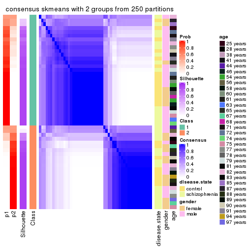
consensus_heatmap(res, k = 3)
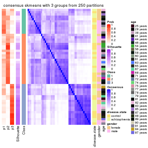
consensus_heatmap(res, k = 4)
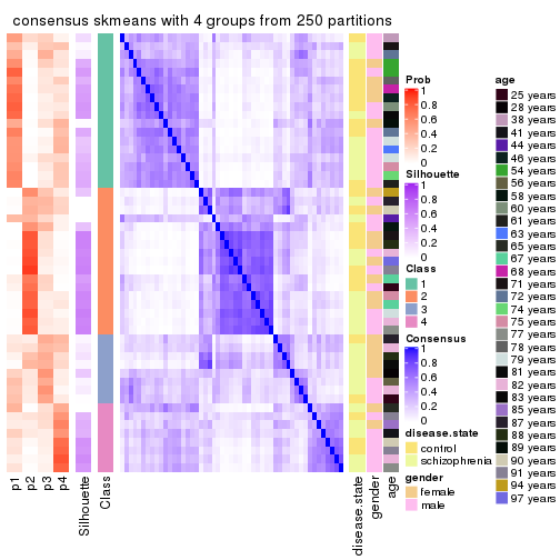
consensus_heatmap(res, k = 5)
consensus_heatmap(res, k = 6)
Heatmaps for the membership of samples in all partitions to see how consistent they are:
membership_heatmap(res, k = 2)
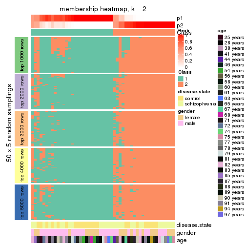
membership_heatmap(res, k = 3)
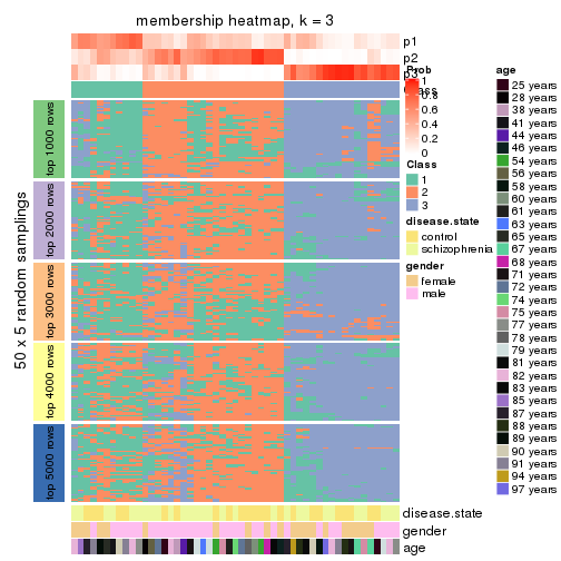
membership_heatmap(res, k = 4)
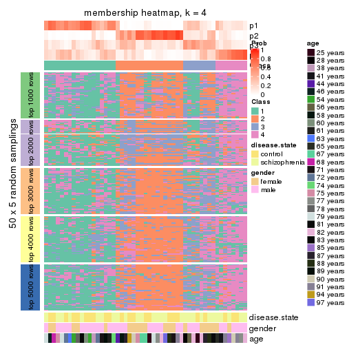
membership_heatmap(res, k = 5)
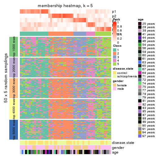
membership_heatmap(res, k = 6)
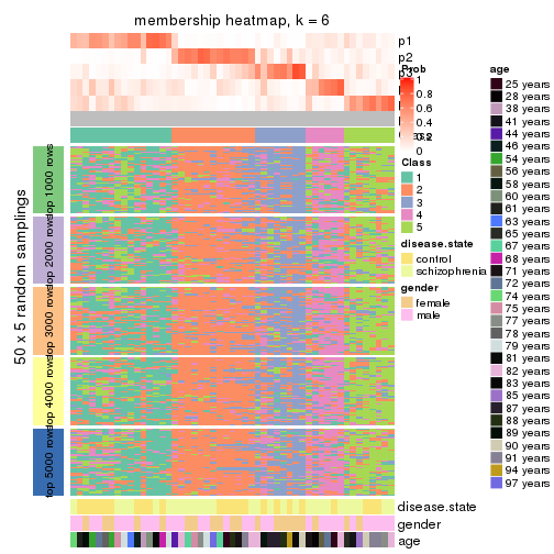
As soon as we have had the classes for columns, we can look for signatures which are significantly different between classes which can be candidate marks for certain classes. Following are the heatmaps for signatures.
Signature heatmaps where rows are scaled:
get_signatures(res, k = 2)
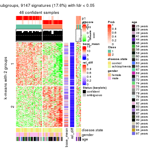
get_signatures(res, k = 3)
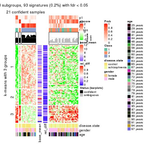
get_signatures(res, k = 4)
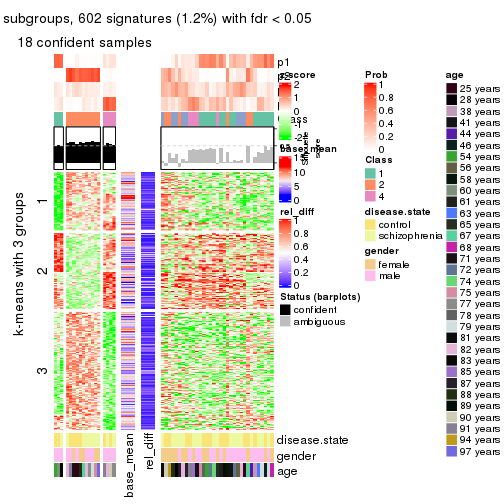
get_signatures(res, k = 5)
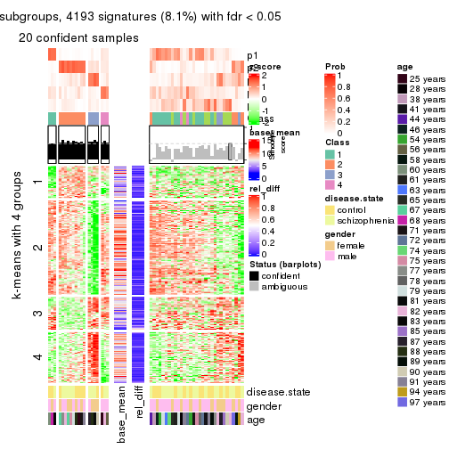
get_signatures(res, k = 6)
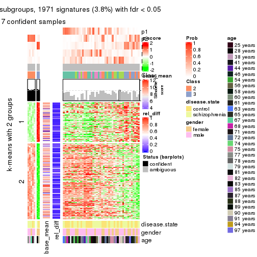
Signature heatmaps where rows are not scaled:
get_signatures(res, k = 2, scale_rows = FALSE)
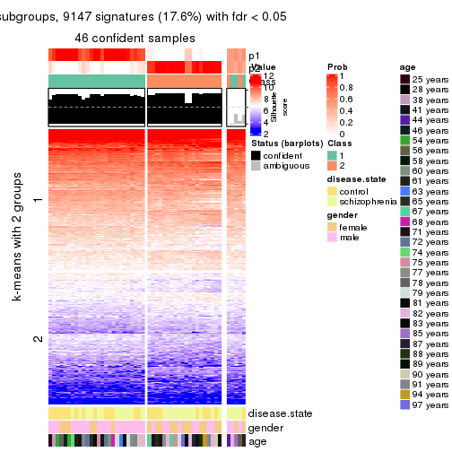
get_signatures(res, k = 3, scale_rows = FALSE)
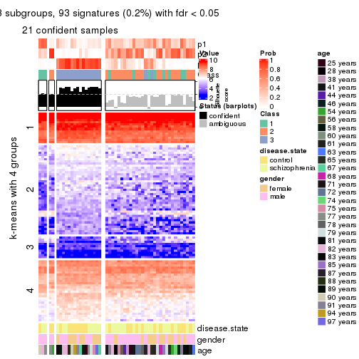
get_signatures(res, k = 4, scale_rows = FALSE)
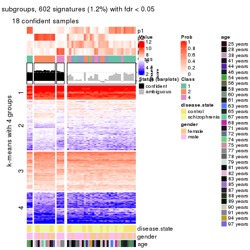
get_signatures(res, k = 5, scale_rows = FALSE)
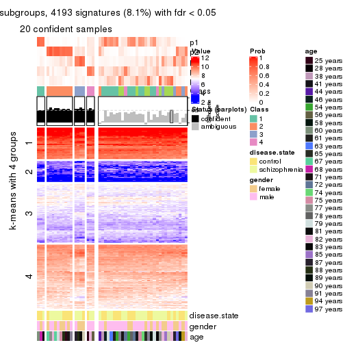
get_signatures(res, k = 6, scale_rows = FALSE)
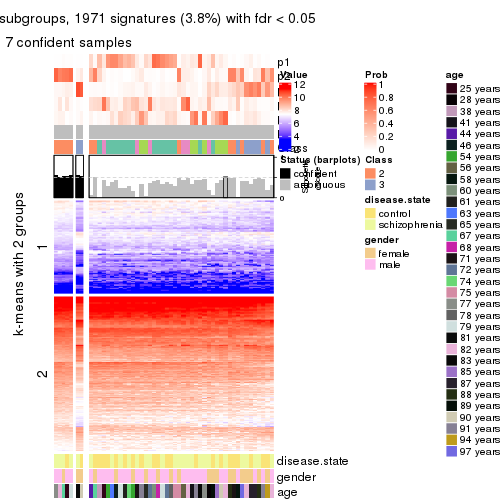
Compare the overlap of signatures from different k:
compare_signatures(res)
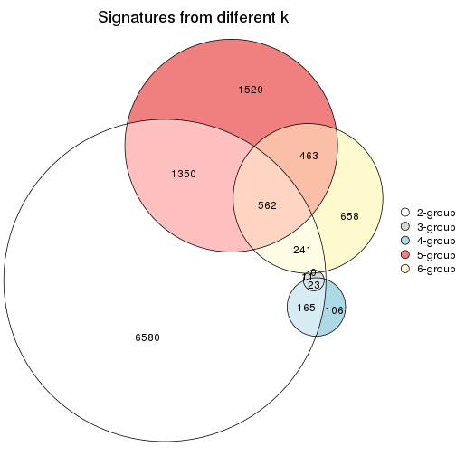
get_signature() returns a data frame invisibly. TO get the list of signatures, the function
call should be assigned to a variable explicitly. In following code, if plot argument is set
to FALSE, no heatmap is plotted while only the differential analysis is performed.
# code only for demonstration
tb = get_signature(res, k = ..., plot = FALSE)
An example of the output of tb is:
#>   which_row         fdr    mean_1    mean_2 scaled_mean_1 scaled_mean_2 km
#> 1        38 0.042760348  8.373488  9.131774    -0.5533452     0.5164555  1
#> 2        40 0.018707592  7.106213  8.469186    -0.6173731     0.5762149  1
#> 3        55 0.019134737 10.221463 11.207825    -0.6159697     0.5749050  1
#> 4        59 0.006059896  5.921854  7.869574    -0.6899429     0.6439467  1
#> 5        60 0.018055526  8.928898 10.211722    -0.6204761     0.5791110  1
#> 6        98 0.009384629 15.714769 14.887706     0.6635654    -0.6193277  2
...
The columns in tb are:
which_row: row indices corresponding to the input matrix.fdr: FDR for the differential test. mean_x: The mean value in group x.scaled_mean_x: The mean value in group x after rows are scaled.km: Row groups if k-means clustering is applied to rows.UMAP plot which shows how samples are separated.
dimension_reduction(res, k = 2, method = "UMAP")
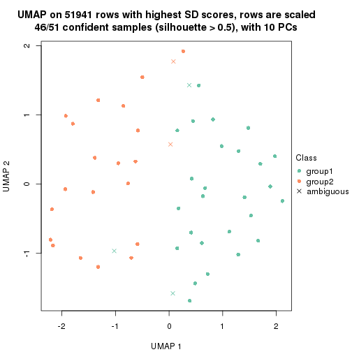
dimension_reduction(res, k = 3, method = "UMAP")
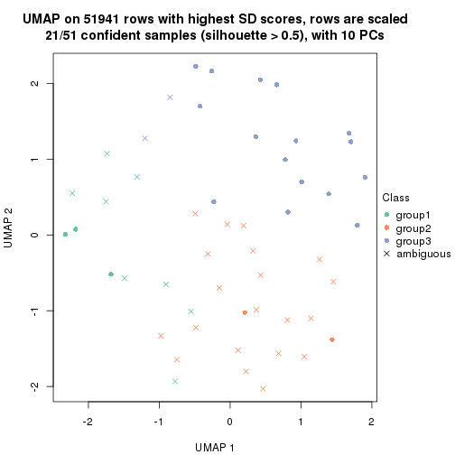
dimension_reduction(res, k = 4, method = "UMAP")
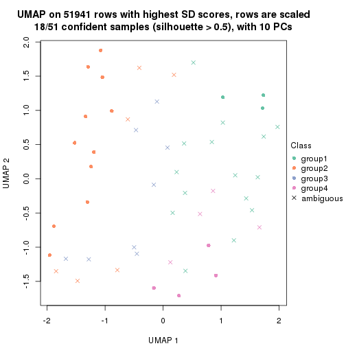
dimension_reduction(res, k = 5, method = "UMAP")
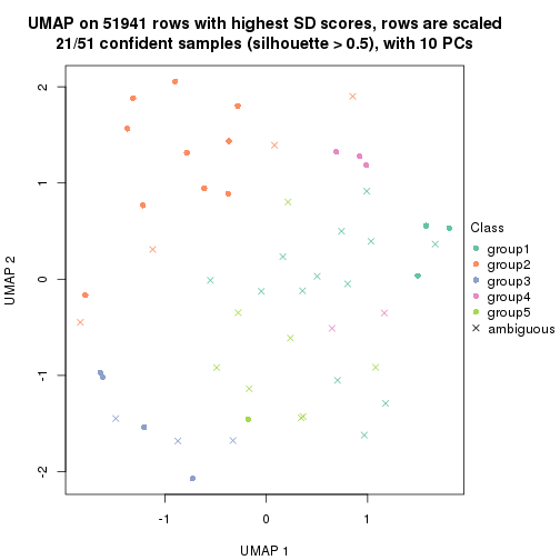
dimension_reduction(res, k = 6, method = "UMAP")
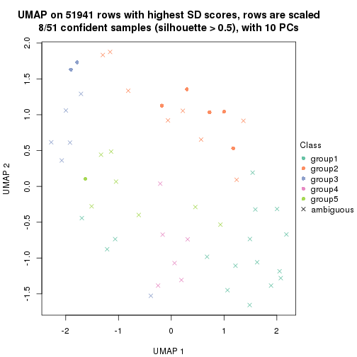
Following heatmap shows how subgroups are split when increasing k:
collect_classes(res)
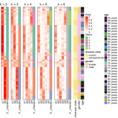
Test correlation between subgroups and known annotations. If the known annotation is numeric, one-way ANOVA test is applied, and if the known annotation is discrete, chi-squared contingency table test is applied.
test_to_known_factors(res)
#>             n disease.state(p) gender(p) age(p) k
#> SD:skmeans 46            0.526    0.0252  0.553 2
#> SD:skmeans 21            0.318    0.0854  0.563 3
#> SD:skmeans 18            0.625    0.1105  0.476 4
#> SD:skmeans 21            0.684    0.2866  0.633 5
#> SD:skmeans  8            0.587    0.1009  0.512 6
If matrix rows can be associated to genes, consider to use functional_enrichment(res,
...) to perform function enrichment for the signature genes. See this vignette for more detailed explanations.
The object with results only for a single top-value method and a single partition method can be extracted as:
res = res_list["SD", "pam"]
# you can also extract it by
# res = res_list["SD:pam"]
A summary of res and all the functions that can be applied to it:
res
#> A 'ConsensusPartition' object with k = 2, 3, 4, 5, 6.
#>   On a matrix with 51941 rows and 51 columns.
#>   Top rows (1000, 2000, 3000, 4000, 5000) are extracted by 'SD' method.
#>   Subgroups are detected by 'pam' method.
#>   Performed in total 1250 partitions by row resampling.
#>   Best k for subgroups seems to be 2.
#>
#> Following methods can be applied to this 'ConsensusPartition' object:
#>  [1] "cola_report"             "collect_classes"         "collect_plots"
#>  [4] "collect_stats"           "colnames"                "compare_signatures"
#>  [7] "consensus_heatmap"       "dimension_reduction"     "functional_enrichment"
#> [10] "get_anno_col"            "get_anno"                "get_classes"
#> [13] "get_consensus"           "get_matrix"              "get_membership"
#> [16] "get_param"               "get_signatures"          "get_stats"
#> [19] "is_best_k"               "is_stable_k"             "membership_heatmap"
#> [22] "ncol"                    "nrow"                    "plot_ecdf"
#> [25] "rownames"                "select_partition_number" "show"
#> [28] "suggest_best_k"          "test_to_known_factors"
collect_plots() function collects all the plots made from res for all k (number of partitions)
into one single page to provide an easy and fast comparison between different k.
collect_plots(res)
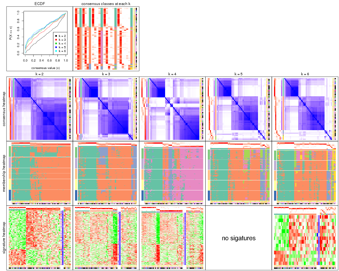
The plots are:
k and the heatmap of
predicted classes for each k.k.k.k.All the plots in panels can be made by individual functions and they are plotted later in this section.
select_partition_number() produces several plots showing different
statistics for choosing “optimized” k. There are following statistics:
k;k, the area increased is defined as \(A_k - A_{k-1}\).The detailed explanations of these statistics can be found in the cola vignette.
Generally speaking, lower PAC score, higher mean silhouette score or higher
concordance corresponds to better partition. Rand index and Jaccard index
measure how similar the current partition is compared to partition with k-1.
If they are too similar, we won't accept k is better than k-1.
select_partition_number(res)
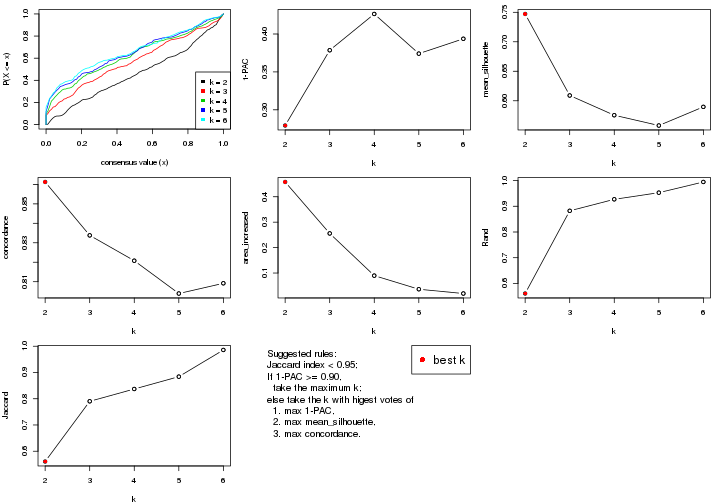
The numeric values for all these statistics can be obtained by get_stats().
get_stats(res)
#>   k 1-PAC mean_silhouette concordance area_increased  Rand Jaccard
#> 2 2 0.279           0.747       0.861         0.4581 0.561   0.561
#> 3 3 0.379           0.609       0.834         0.2557 0.882   0.790
#> 4 4 0.426           0.575       0.821         0.0899 0.927   0.837
#> 5 5 0.374           0.558       0.804         0.0364 0.953   0.884
#> 6 6 0.394           0.590       0.809         0.0195 0.995   0.986
suggest_best_k() suggests the best \(k\) based on these statistics. The rules are as follows:
suggest_best_k(res)
#> [1] 2
Following shows the table of the partitions (You need to click the show/hide
code output link to see it). The membership matrix (columns with name p*)
is inferred by
clue::cl_consensus()
function with the SE method. Basically the value in the membership matrix
represents the probability to belong to a certain group. The finall class
label for an item is determined with the group with highest probability it
belongs to.
In get_classes() function, the entropy is calculated from the membership
matrix and the silhouette score is calculated from the consensus matrix.
cbind(get_classes(res, k = 2), get_membership(res, k = 2))
#>           class entropy silhouette    p1    p2
#> GSM439800     1  0.9170      0.463 0.668 0.332
#> GSM439790     2  0.4562      0.836 0.096 0.904
#> GSM439827     2  0.1414      0.826 0.020 0.980
#> GSM439811     2  0.2778      0.821 0.048 0.952
#> GSM439795     2  0.7376      0.778 0.208 0.792
#> GSM439805     2  0.4690      0.836 0.100 0.900
#> GSM439781     2  0.9881      0.239 0.436 0.564
#> GSM439807     1  0.6801      0.770 0.820 0.180
#> GSM439820     2  0.1414      0.824 0.020 0.980
#> GSM439784     1  0.2043      0.873 0.968 0.032
#> GSM439824     2  0.4022      0.841 0.080 0.920
#> GSM439794     2  0.5408      0.830 0.124 0.876
#> GSM439809     1  0.6712      0.789 0.824 0.176
#> GSM439785     2  0.4161      0.834 0.084 0.916
#> GSM439803     2  0.4939      0.836 0.108 0.892
#> GSM439778     1  0.6801      0.787 0.820 0.180
#> GSM439791     2  0.5178      0.834 0.116 0.884
#> GSM439786     2  0.4815      0.837 0.104 0.896
#> GSM439828     2  0.0376      0.830 0.004 0.996
#> GSM439806     1  0.9286      0.528 0.656 0.344
#> GSM439815     2  0.7745      0.734 0.228 0.772
#> GSM439817     2  0.9358      0.453 0.352 0.648
#> GSM439796     2  0.4161      0.834 0.084 0.916
#> GSM439798     2  0.8144      0.719 0.252 0.748
#> GSM439821     2  0.1184      0.826 0.016 0.984
#> GSM439823     2  0.0672      0.831 0.008 0.992
#> GSM439813     1  0.1414      0.871 0.980 0.020
#> GSM439801     2  0.3733      0.839 0.072 0.928
#> GSM439810     2  0.8386      0.694 0.268 0.732
#> GSM439783     2  0.9970      0.227 0.468 0.532
#> GSM439826     2  0.0376      0.830 0.004 0.996
#> GSM439812     1  0.1414      0.871 0.980 0.020
#> GSM439818     2  0.2778      0.822 0.048 0.952
#> GSM439792     1  0.1184      0.871 0.984 0.016
#> GSM439802     1  0.0938      0.865 0.988 0.012
#> GSM439825     2  0.0938      0.825 0.012 0.988
#> GSM439780     1  0.0672      0.867 0.992 0.008
#> GSM439787     2  0.9963      0.111 0.464 0.536
#> GSM439808     2  0.9795      0.285 0.416 0.584
#> GSM439804     2  0.4939      0.835 0.108 0.892
#> GSM439822     2  0.5737      0.796 0.136 0.864
#> GSM439816     2  0.9248      0.591 0.340 0.660
#> GSM439789     1  0.2423      0.870 0.960 0.040
#> GSM439799     2  0.0938      0.832 0.012 0.988
#> GSM439814     1  0.2423      0.870 0.960 0.040
#> GSM439782     2  0.8499      0.661 0.276 0.724
#> GSM439779     1  0.1633      0.872 0.976 0.024
#> GSM439793     1  0.6887      0.771 0.816 0.184
#> GSM439788     1  0.7139      0.765 0.804 0.196
#> GSM439797     2  0.4161      0.834 0.084 0.916
#> GSM439819     2  0.2043      0.822 0.032 0.968
cbind(get_classes(res, k = 3), get_membership(res, k = 3))
#>           class entropy silhouette    p1    p2    p3
#> GSM439800     1  0.5929     0.4561 0.676 0.320 0.004
#> GSM439790     2  0.1031     0.7408 0.024 0.976 0.000
#> GSM439827     2  0.5785     0.4259 0.000 0.668 0.332
#> GSM439811     2  0.5988     0.3587 0.000 0.632 0.368
#> GSM439795     3  0.7979     0.5384 0.100 0.272 0.628
#> GSM439805     2  0.0747     0.7407 0.016 0.984 0.000
#> GSM439781     2  0.9390     0.1449 0.320 0.488 0.192
#> GSM439807     1  0.8158     0.2779 0.556 0.080 0.364
#> GSM439820     2  0.5621     0.4640 0.000 0.692 0.308
#> GSM439784     1  0.0747     0.8265 0.984 0.016 0.000
#> GSM439824     2  0.0983     0.7402 0.016 0.980 0.004
#> GSM439794     2  0.2165     0.7302 0.064 0.936 0.000
#> GSM439809     1  0.4062     0.7320 0.836 0.164 0.000
#> GSM439785     2  0.0000     0.7351 0.000 1.000 0.000
#> GSM439803     2  0.1031     0.7410 0.024 0.976 0.000
#> GSM439778     1  0.4002     0.7389 0.840 0.160 0.000
#> GSM439791     2  0.2066     0.7326 0.060 0.940 0.000
#> GSM439786     2  0.0424     0.7383 0.008 0.992 0.000
#> GSM439828     2  0.2448     0.7156 0.000 0.924 0.076
#> GSM439806     1  0.6140     0.3477 0.596 0.404 0.000
#> GSM439815     2  0.3752     0.6347 0.144 0.856 0.000
#> GSM439817     2  0.9092     0.2321 0.296 0.532 0.172
#> GSM439796     2  0.0000     0.7351 0.000 1.000 0.000
#> GSM439798     2  0.3941     0.6268 0.156 0.844 0.000
#> GSM439821     3  0.5835     0.5212 0.000 0.340 0.660
#> GSM439823     2  0.1163     0.7349 0.000 0.972 0.028
#> GSM439813     1  0.0000     0.8300 1.000 0.000 0.000
#> GSM439801     2  0.0237     0.7356 0.000 0.996 0.004
#> GSM439810     2  0.4399     0.6035 0.188 0.812 0.000
#> GSM439783     2  0.6305     0.0628 0.484 0.516 0.000
#> GSM439826     2  0.2796     0.7070 0.000 0.908 0.092
#> GSM439812     1  0.0000     0.8300 1.000 0.000 0.000
#> GSM439818     2  0.6379     0.3583 0.008 0.624 0.368
#> GSM439792     1  0.0000     0.8300 1.000 0.000 0.000
#> GSM439802     1  0.0747     0.8231 0.984 0.000 0.016
#> GSM439825     2  0.6111     0.3004 0.000 0.604 0.396
#> GSM439780     1  0.0000     0.8300 1.000 0.000 0.000
#> GSM439787     3  0.3530     0.6053 0.032 0.068 0.900
#> GSM439808     3  0.5470     0.6114 0.036 0.168 0.796
#> GSM439804     2  0.2066     0.7326 0.060 0.940 0.000
#> GSM439822     2  0.7944     0.4432 0.112 0.644 0.244
#> GSM439816     2  0.5835     0.4236 0.340 0.660 0.000
#> GSM439789     1  0.0000     0.8300 1.000 0.000 0.000
#> GSM439799     2  0.0237     0.7356 0.000 0.996 0.004
#> GSM439814     1  0.0000     0.8300 1.000 0.000 0.000
#> GSM439782     2  0.4504     0.5634 0.196 0.804 0.000
#> GSM439779     1  0.0000     0.8300 1.000 0.000 0.000
#> GSM439793     1  0.4178     0.7173 0.828 0.172 0.000
#> GSM439788     1  0.4504     0.7043 0.804 0.196 0.000
#> GSM439797     2  0.0000     0.7351 0.000 1.000 0.000
#> GSM439819     3  0.6280    -0.0283 0.000 0.460 0.540
cbind(get_classes(res, k = 4), get_membership(res, k = 4))
#>           class entropy silhouette    p1    p2    p3    p4
#> GSM439800     1  0.4699    0.48375 0.676 0.000 0.004 0.320
#> GSM439790     4  0.1004    0.73414 0.024 0.004 0.000 0.972
#> GSM439827     4  0.4999   -0.41976 0.000 0.492 0.000 0.508
#> GSM439811     2  0.5167    0.30722 0.000 0.508 0.004 0.488
#> GSM439795     3  0.1520    0.83532 0.000 0.020 0.956 0.024
#> GSM439805     4  0.0592    0.73267 0.016 0.000 0.000 0.984
#> GSM439781     4  0.7550    0.00115 0.300 0.220 0.000 0.480
#> GSM439807     1  0.8748    0.16604 0.464 0.252 0.220 0.064
#> GSM439820     4  0.5004   -0.03079 0.000 0.392 0.004 0.604
#> GSM439784     1  0.0592    0.81921 0.984 0.000 0.000 0.016
#> GSM439824     4  0.0779    0.73313 0.016 0.004 0.000 0.980
#> GSM439794     4  0.1716    0.72737 0.064 0.000 0.000 0.936
#> GSM439809     1  0.3219    0.74864 0.836 0.000 0.000 0.164
#> GSM439785     4  0.0000    0.72510 0.000 0.000 0.000 1.000
#> GSM439803     4  0.0817    0.73445 0.024 0.000 0.000 0.976
#> GSM439778     1  0.3172    0.74972 0.840 0.000 0.000 0.160
#> GSM439791     4  0.1637    0.72770 0.060 0.000 0.000 0.940
#> GSM439786     4  0.0336    0.72972 0.008 0.000 0.000 0.992
#> GSM439828     4  0.2149    0.68960 0.000 0.088 0.000 0.912
#> GSM439806     1  0.4866    0.37559 0.596 0.000 0.000 0.404
#> GSM439815     4  0.2973    0.64568 0.144 0.000 0.000 0.856
#> GSM439817     4  0.7382    0.04756 0.260 0.220 0.000 0.520
#> GSM439796     4  0.0000    0.72510 0.000 0.000 0.000 1.000
#> GSM439798     4  0.3123    0.63591 0.156 0.000 0.000 0.844
#> GSM439821     3  0.4741    0.74209 0.000 0.228 0.744 0.028
#> GSM439823     4  0.1022    0.72248 0.000 0.032 0.000 0.968
#> GSM439813     1  0.0000    0.82118 1.000 0.000 0.000 0.000
#> GSM439801     4  0.2281    0.69317 0.000 0.000 0.096 0.904
#> GSM439810     4  0.3486    0.60934 0.188 0.000 0.000 0.812
#> GSM439783     4  0.4996    0.08606 0.484 0.000 0.000 0.516
#> GSM439826     4  0.2760    0.65202 0.000 0.128 0.000 0.872
#> GSM439812     1  0.0000    0.82118 1.000 0.000 0.000 0.000
#> GSM439818     2  0.4088    0.55472 0.000 0.764 0.004 0.232
#> GSM439792     1  0.0000    0.82118 1.000 0.000 0.000 0.000
#> GSM439802     1  0.2081    0.77015 0.916 0.000 0.084 0.000
#> GSM439825     2  0.5508    0.49779 0.000 0.572 0.020 0.408
#> GSM439780     1  0.0000    0.82118 1.000 0.000 0.000 0.000
#> GSM439787     3  0.2221    0.84400 0.016 0.008 0.932 0.044
#> GSM439808     2  0.6925    0.12789 0.008 0.520 0.384 0.088
#> GSM439804     4  0.1637    0.72760 0.060 0.000 0.000 0.940
#> GSM439822     4  0.6795   -0.28143 0.084 0.412 0.004 0.500
#> GSM439816     4  0.4624    0.42186 0.340 0.000 0.000 0.660
#> GSM439789     1  0.0000    0.82118 1.000 0.000 0.000 0.000
#> GSM439799     4  0.2281    0.69317 0.000 0.000 0.096 0.904
#> GSM439814     1  0.0000    0.82118 1.000 0.000 0.000 0.000
#> GSM439782     4  0.3569    0.57430 0.196 0.000 0.000 0.804
#> GSM439779     1  0.0000    0.82118 1.000 0.000 0.000 0.000
#> GSM439793     1  0.3311    0.73306 0.828 0.000 0.000 0.172
#> GSM439788     1  0.3569    0.72400 0.804 0.000 0.000 0.196
#> GSM439797     4  0.0000    0.72510 0.000 0.000 0.000 1.000
#> GSM439819     2  0.6854    0.35772 0.000 0.600 0.196 0.204
cbind(get_classes(res, k = 5), get_membership(res, k = 5))
#>           class entropy silhouette    p1    p2    p3    p4    p5
#> GSM439800     1  0.6108     0.3011 0.548 0.316 0.000 0.004 0.132
#> GSM439790     2  0.0865     0.7656 0.024 0.972 0.000 0.004 0.000
#> GSM439827     2  0.4893     0.3480 0.000 0.568 0.000 0.404 0.028
#> GSM439811     2  0.4982     0.3274 0.000 0.556 0.000 0.412 0.032
#> GSM439795     3  0.0290     0.3108 0.000 0.008 0.992 0.000 0.000
#> GSM439805     2  0.0671     0.7635 0.016 0.980 0.000 0.000 0.004
#> GSM439781     2  0.6595     0.2938 0.296 0.488 0.000 0.212 0.004
#> GSM439807     3  0.8405     0.0628 0.324 0.056 0.352 0.232 0.036
#> GSM439820     2  0.4934     0.4203 0.000 0.600 0.000 0.364 0.036
#> GSM439784     1  0.0510     0.8234 0.984 0.016 0.000 0.000 0.000
#> GSM439824     2  0.0960     0.7648 0.016 0.972 0.000 0.004 0.008
#> GSM439794     2  0.2344     0.7626 0.032 0.904 0.000 0.000 0.064
#> GSM439809     1  0.2773     0.7346 0.836 0.164 0.000 0.000 0.000
#> GSM439785     2  0.0000     0.7551 0.000 1.000 0.000 0.000 0.000
#> GSM439803     2  0.1800     0.7648 0.020 0.932 0.000 0.000 0.048
#> GSM439778     1  0.2732     0.7369 0.840 0.160 0.000 0.000 0.000
#> GSM439791     2  0.1410     0.7640 0.060 0.940 0.000 0.000 0.000
#> GSM439786     2  0.0579     0.7609 0.008 0.984 0.000 0.000 0.008
#> GSM439828     2  0.2331     0.7471 0.000 0.900 0.000 0.080 0.020
#> GSM439806     1  0.4192     0.3964 0.596 0.404 0.000 0.000 0.000
#> GSM439815     2  0.2719     0.6918 0.144 0.852 0.000 0.000 0.004
#> GSM439817     2  0.6624     0.3406 0.264 0.516 0.004 0.212 0.004
#> GSM439796     2  0.1732     0.7566 0.000 0.920 0.000 0.000 0.080
#> GSM439798     2  0.2971     0.6796 0.156 0.836 0.000 0.000 0.008
#> GSM439821     5  0.4291    -0.1294 0.000 0.000 0.464 0.000 0.536
#> GSM439823     2  0.1568     0.7605 0.000 0.944 0.000 0.036 0.020
#> GSM439813     1  0.0290     0.8240 0.992 0.000 0.000 0.000 0.008
#> GSM439801     2  0.1965     0.7447 0.000 0.904 0.096 0.000 0.000
#> GSM439810     2  0.3391     0.6628 0.188 0.800 0.000 0.000 0.012
#> GSM439783     2  0.4448     0.1143 0.480 0.516 0.000 0.000 0.004
#> GSM439826     2  0.4313     0.6448 0.000 0.732 0.000 0.040 0.228
#> GSM439812     1  0.0162     0.8244 0.996 0.000 0.000 0.000 0.004
#> GSM439818     4  0.2561     0.0000 0.000 0.020 0.000 0.884 0.096
#> GSM439792     1  0.0162     0.8244 0.996 0.000 0.000 0.000 0.004
#> GSM439802     1  0.2011     0.7651 0.908 0.000 0.088 0.000 0.004
#> GSM439825     5  0.7023    -0.0761 0.000 0.348 0.008 0.280 0.364
#> GSM439780     1  0.0000     0.8242 1.000 0.000 0.000 0.000 0.000
#> GSM439787     3  0.3042     0.2637 0.020 0.044 0.880 0.000 0.056
#> GSM439808     3  0.7017    -0.1446 0.008 0.076 0.440 0.416 0.060
#> GSM439804     2  0.2561     0.7533 0.020 0.884 0.000 0.000 0.096
#> GSM439822     2  0.6666     0.2458 0.016 0.496 0.000 0.160 0.328
#> GSM439816     2  0.4969     0.5407 0.292 0.652 0.000 0.000 0.056
#> GSM439789     1  0.0290     0.8240 0.992 0.000 0.000 0.000 0.008
#> GSM439799     2  0.2623     0.7407 0.000 0.884 0.096 0.004 0.016
#> GSM439814     1  0.0000     0.8242 1.000 0.000 0.000 0.000 0.000
#> GSM439782     2  0.3074     0.6276 0.196 0.804 0.000 0.000 0.000
#> GSM439779     1  0.0000     0.8242 1.000 0.000 0.000 0.000 0.000
#> GSM439793     1  0.2852     0.7172 0.828 0.172 0.000 0.000 0.000
#> GSM439788     1  0.3074     0.7068 0.804 0.196 0.000 0.000 0.000
#> GSM439797     2  0.0000     0.7551 0.000 1.000 0.000 0.000 0.000
#> GSM439819     5  0.7175    -0.0768 0.000 0.068 0.140 0.276 0.516
cbind(get_classes(res, k = 6), get_membership(res, k = 6))
#>           class entropy silhouette    p1    p2    p3    p4    p5    p6
#> GSM439800     1  0.7517      0.192 0.460 0.276 0.012 0.080 0.144 0.028
#> GSM439790     2  0.0777      0.788 0.024 0.972 0.000 0.000 0.004 0.000
#> GSM439827     2  0.5386      0.576 0.000 0.648 0.212 0.104 0.036 0.000
#> GSM439811     2  0.5409      0.567 0.000 0.640 0.220 0.108 0.032 0.000
#> GSM439795     3  0.4372     -0.261 0.000 0.000 0.544 0.024 0.000 0.432
#> GSM439805     2  0.0603      0.786 0.016 0.980 0.000 0.004 0.000 0.000
#> GSM439781     2  0.6923      0.353 0.292 0.488 0.112 0.092 0.016 0.000
#> GSM439807     3  0.4085      0.261 0.252 0.044 0.704 0.000 0.000 0.000
#> GSM439820     2  0.5996      0.566 0.000 0.636 0.192 0.100 0.036 0.036
#> GSM439784     1  0.0458      0.818 0.984 0.016 0.000 0.000 0.000 0.000
#> GSM439824     2  0.0862      0.787 0.016 0.972 0.004 0.008 0.000 0.000
#> GSM439794     2  0.2285      0.786 0.028 0.900 0.000 0.008 0.064 0.000
#> GSM439809     1  0.2491      0.729 0.836 0.164 0.000 0.000 0.000 0.000
#> GSM439785     2  0.0000      0.778 0.000 1.000 0.000 0.000 0.000 0.000
#> GSM439803     2  0.1616      0.789 0.020 0.932 0.000 0.000 0.048 0.000
#> GSM439778     1  0.2454      0.730 0.840 0.160 0.000 0.000 0.000 0.000
#> GSM439791     2  0.1267      0.788 0.060 0.940 0.000 0.000 0.000 0.000
#> GSM439786     2  0.1728      0.782 0.004 0.924 0.000 0.064 0.008 0.000
#> GSM439828     2  0.2544      0.776 0.000 0.896 0.048 0.024 0.028 0.004
#> GSM439806     1  0.3765      0.398 0.596 0.404 0.000 0.000 0.000 0.000
#> GSM439815     2  0.2442      0.721 0.144 0.852 0.000 0.000 0.004 0.000
#> GSM439817     2  0.7088      0.408 0.264 0.516 0.100 0.076 0.040 0.004
#> GSM439796     2  0.1700      0.782 0.000 0.916 0.000 0.004 0.080 0.000
#> GSM439798     2  0.3930      0.688 0.156 0.772 0.000 0.064 0.008 0.000
#> GSM439821     6  0.2766      0.405 0.000 0.000 0.028 0.092 0.012 0.868
#> GSM439823     2  0.1690      0.785 0.000 0.940 0.020 0.016 0.020 0.004
#> GSM439813     1  0.0260      0.819 0.992 0.000 0.000 0.000 0.008 0.000
#> GSM439801     2  0.1863      0.772 0.000 0.896 0.000 0.000 0.000 0.104
#> GSM439810     2  0.3089      0.692 0.188 0.800 0.000 0.004 0.008 0.000
#> GSM439783     2  0.3995      0.134 0.480 0.516 0.000 0.004 0.000 0.000
#> GSM439826     2  0.4427      0.631 0.000 0.676 0.016 0.016 0.284 0.008
#> GSM439812     1  0.0146      0.819 0.996 0.000 0.000 0.004 0.000 0.000
#> GSM439818     5  0.3412      0.000 0.000 0.000 0.128 0.064 0.808 0.000
#> GSM439792     1  0.0146      0.819 0.996 0.000 0.000 0.004 0.000 0.000
#> GSM439802     1  0.2398      0.747 0.888 0.000 0.028 0.004 0.000 0.080
#> GSM439825     4  0.3400      0.000 0.000 0.064 0.092 0.832 0.008 0.004
#> GSM439780     1  0.0000      0.819 1.000 0.000 0.000 0.000 0.000 0.000
#> GSM439787     6  0.6088     -0.157 0.032 0.056 0.408 0.028 0.000 0.476
#> GSM439808     3  0.2775      0.234 0.008 0.076 0.880 0.008 0.024 0.004
#> GSM439804     2  0.2555      0.779 0.020 0.876 0.000 0.008 0.096 0.000
#> GSM439822     2  0.7093      0.307 0.004 0.484 0.064 0.040 0.308 0.100
#> GSM439816     2  0.4626      0.584 0.292 0.652 0.000 0.012 0.044 0.000
#> GSM439789     1  0.0260      0.819 0.992 0.000 0.000 0.000 0.008 0.000
#> GSM439799     2  0.2266      0.770 0.000 0.880 0.000 0.000 0.012 0.108
#> GSM439814     1  0.0000      0.819 1.000 0.000 0.000 0.000 0.000 0.000
#> GSM439782     2  0.2762      0.657 0.196 0.804 0.000 0.000 0.000 0.000
#> GSM439779     1  0.0000      0.819 1.000 0.000 0.000 0.000 0.000 0.000
#> GSM439793     1  0.2562      0.712 0.828 0.172 0.000 0.000 0.000 0.000
#> GSM439788     1  0.2762      0.701 0.804 0.196 0.000 0.000 0.000 0.000
#> GSM439797     2  0.0000      0.778 0.000 1.000 0.000 0.000 0.000 0.000
#> GSM439819     6  0.5702      0.222 0.000 0.032 0.148 0.104 0.040 0.676
Heatmaps for the consensus matrix. It visualizes the probability of two samples to be in a same group.
consensus_heatmap(res, k = 2)
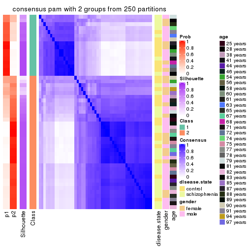
consensus_heatmap(res, k = 3)
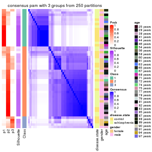
consensus_heatmap(res, k = 4)
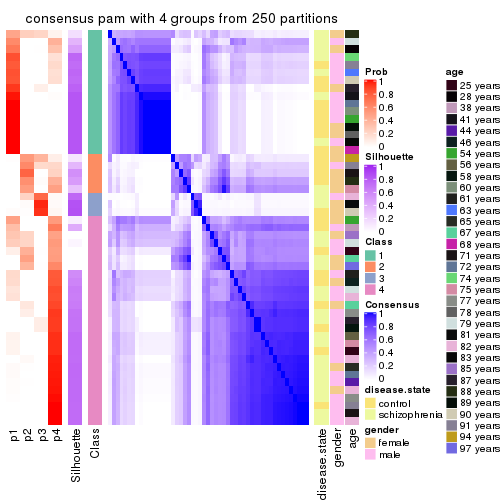
consensus_heatmap(res, k = 5)
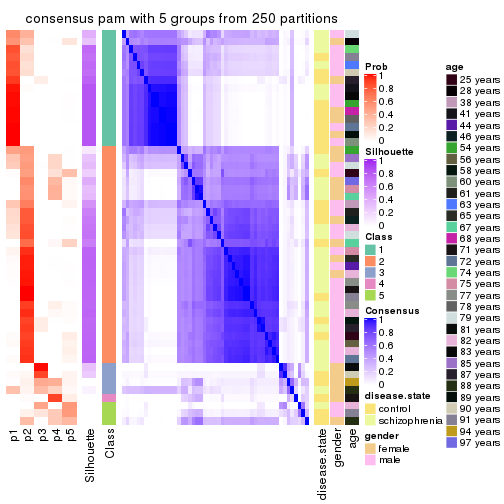
consensus_heatmap(res, k = 6)
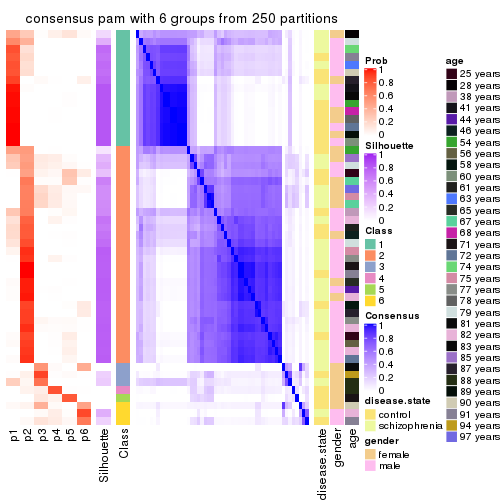
Heatmaps for the membership of samples in all partitions to see how consistent they are:
membership_heatmap(res, k = 2)
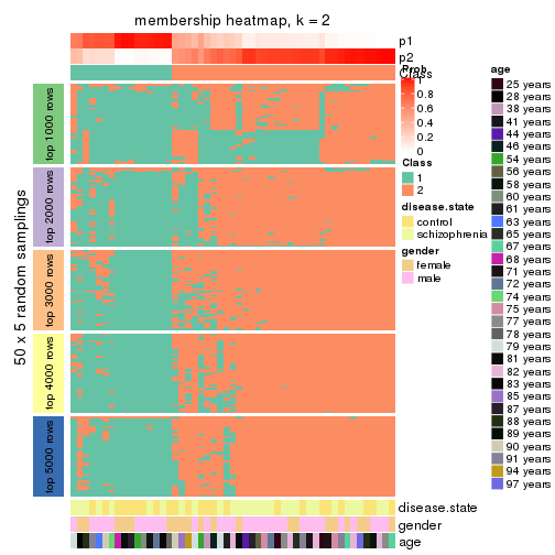
membership_heatmap(res, k = 3)
membership_heatmap(res, k = 4)
membership_heatmap(res, k = 5)
membership_heatmap(res, k = 6)
As soon as we have had the classes for columns, we can look for signatures which are significantly different between classes which can be candidate marks for certain classes. Following are the heatmaps for signatures.
Signature heatmaps where rows are scaled:
get_signatures(res, k = 2)
get_signatures(res, k = 3)
get_signatures(res, k = 4)
get_signatures(res, k = 5)

get_signatures(res, k = 6)
Signature heatmaps where rows are not scaled:
get_signatures(res, k = 2, scale_rows = FALSE)
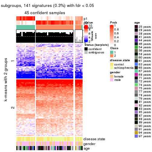
get_signatures(res, k = 3, scale_rows = FALSE)
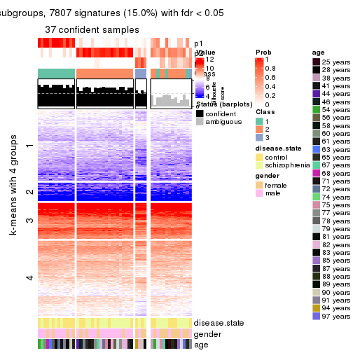
get_signatures(res, k = 4, scale_rows = FALSE)
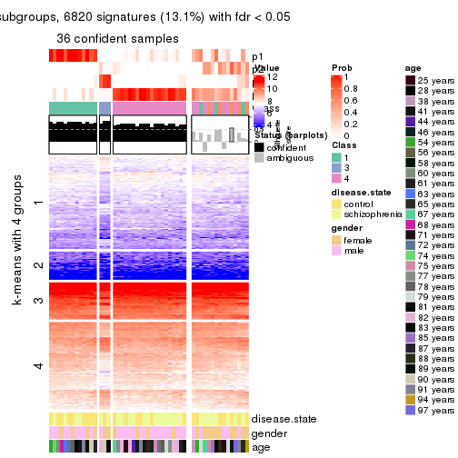
get_signatures(res, k = 5, scale_rows = FALSE)

get_signatures(res, k = 6, scale_rows = FALSE)
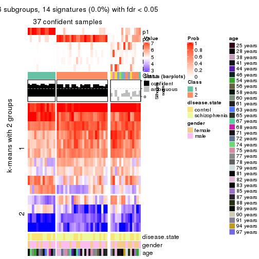
Compare the overlap of signatures from different k:
compare_signatures(res)
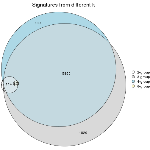
get_signature() returns a data frame invisibly. TO get the list of signatures, the function
call should be assigned to a variable explicitly. In following code, if plot argument is set
to FALSE, no heatmap is plotted while only the differential analysis is performed.
# code only for demonstration
tb = get_signature(res, k = ..., plot = FALSE)
An example of the output of tb is:
#>   which_row         fdr    mean_1    mean_2 scaled_mean_1 scaled_mean_2 km
#> 1        38 0.042760348  8.373488  9.131774    -0.5533452     0.5164555  1
#> 2        40 0.018707592  7.106213  8.469186    -0.6173731     0.5762149  1
#> 3        55 0.019134737 10.221463 11.207825    -0.6159697     0.5749050  1
#> 4        59 0.006059896  5.921854  7.869574    -0.6899429     0.6439467  1
#> 5        60 0.018055526  8.928898 10.211722    -0.6204761     0.5791110  1
#> 6        98 0.009384629 15.714769 14.887706     0.6635654    -0.6193277  2
...
The columns in tb are:
which_row: row indices corresponding to the input matrix.fdr: FDR for the differential test. mean_x: The mean value in group x.scaled_mean_x: The mean value in group x after rows are scaled.km: Row groups if k-means clustering is applied to rows.UMAP plot which shows how samples are separated.
dimension_reduction(res, k = 2, method = "UMAP")
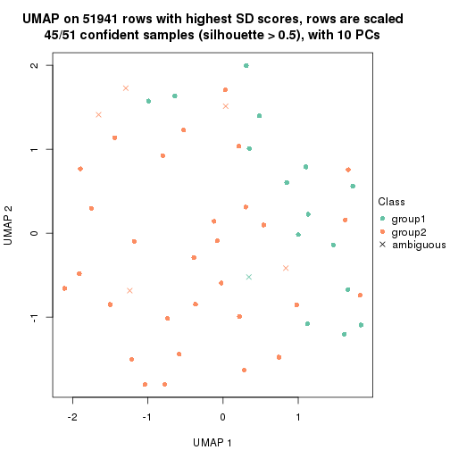
dimension_reduction(res, k = 3, method = "UMAP")

dimension_reduction(res, k = 4, method = "UMAP")
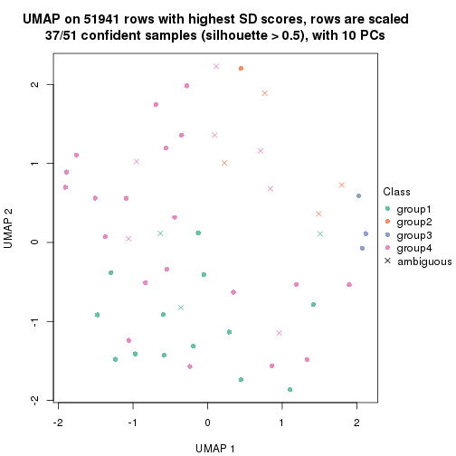
dimension_reduction(res, k = 5, method = "UMAP")
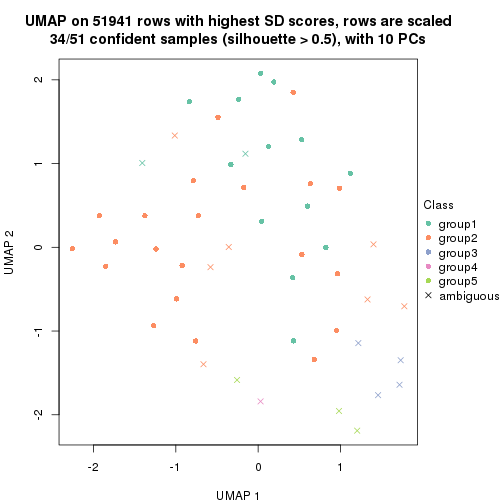
dimension_reduction(res, k = 6, method = "UMAP")
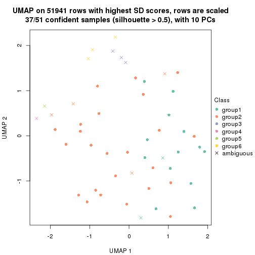
Following heatmap shows how subgroups are split when increasing k:
collect_classes(res)

Test correlation between subgroups and known annotations. If the known annotation is numeric, one-way ANOVA test is applied, and if the known annotation is discrete, chi-squared contingency table test is applied.
test_to_known_factors(res)
#>         n disease.state(p) gender(p) age(p) k
#> SD:pam 45           0.2433    1.0000  0.278 2
#> SD:pam 37           0.0858    0.0891  0.551 3
#> SD:pam 37           0.0999    0.1553  0.841 4
#> SD:pam 34           0.0921    0.7136  0.376 5
#> SD:pam 37           0.0454    1.0000  0.296 6
If matrix rows can be associated to genes, consider to use functional_enrichment(res,
...) to perform function enrichment for the signature genes. See this vignette for more detailed explanations.
The object with results only for a single top-value method and a single partition method can be extracted as:
res = res_list["SD", "mclust"]
# you can also extract it by
# res = res_list["SD:mclust"]
A summary of res and all the functions that can be applied to it:
res
#> A 'ConsensusPartition' object with k = 2, 3, 4, 5, 6.
#>   On a matrix with 51941 rows and 51 columns.
#>   Top rows (1000, 2000, 3000, 4000, 5000) are extracted by 'SD' method.
#>   Subgroups are detected by 'mclust' method.
#>   Performed in total 1250 partitions by row resampling.
#>   Best k for subgroups seems to be 5.
#>
#> Following methods can be applied to this 'ConsensusPartition' object:
#>  [1] "cola_report"             "collect_classes"         "collect_plots"
#>  [4] "collect_stats"           "colnames"                "compare_signatures"
#>  [7] "consensus_heatmap"       "dimension_reduction"     "functional_enrichment"
#> [10] "get_anno_col"            "get_anno"                "get_classes"
#> [13] "get_consensus"           "get_matrix"              "get_membership"
#> [16] "get_param"               "get_signatures"          "get_stats"
#> [19] "is_best_k"               "is_stable_k"             "membership_heatmap"
#> [22] "ncol"                    "nrow"                    "plot_ecdf"
#> [25] "rownames"                "select_partition_number" "show"
#> [28] "suggest_best_k"          "test_to_known_factors"
collect_plots() function collects all the plots made from res for all k (number of partitions)
into one single page to provide an easy and fast comparison between different k.
collect_plots(res)
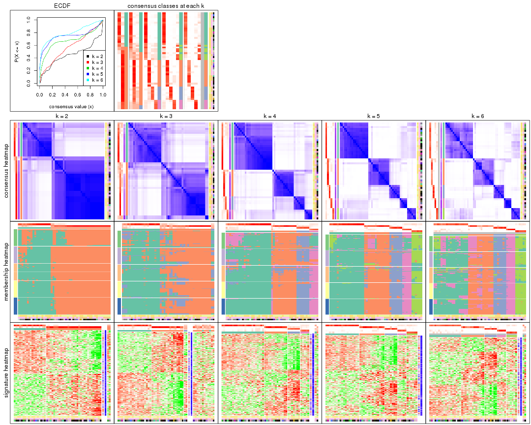
The plots are:
k and the heatmap of
predicted classes for each k.k.k.k.All the plots in panels can be made by individual functions and they are plotted later in this section.
select_partition_number() produces several plots showing different
statistics for choosing “optimized” k. There are following statistics:
k;k, the area increased is defined as \(A_k - A_{k-1}\).The detailed explanations of these statistics can be found in the cola vignette.
Generally speaking, lower PAC score, higher mean silhouette score or higher
concordance corresponds to better partition. Rand index and Jaccard index
measure how similar the current partition is compared to partition with k-1.
If they are too similar, we won't accept k is better than k-1.
select_partition_number(res)
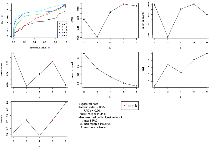
The numeric values for all these statistics can be obtained by get_stats().
get_stats(res)
#>   k 1-PAC mean_silhouette concordance area_increased  Rand Jaccard
#> 2 2 0.540           0.843       0.915         0.4523 0.534   0.534
#> 3 3 0.356           0.533       0.795         0.2720 0.843   0.728
#> 4 4 0.613           0.804       0.839         0.1782 0.728   0.489
#> 5 5 0.697           0.852       0.885         0.1041 0.911   0.730
#> 6 6 0.678           0.752       0.799         0.0666 1.000   1.000
suggest_best_k() suggests the best \(k\) based on these statistics. The rules are as follows:
suggest_best_k(res)
#> [1] 5
Following shows the table of the partitions (You need to click the show/hide
code output link to see it). The membership matrix (columns with name p*)
is inferred by
clue::cl_consensus()
function with the SE method. Basically the value in the membership matrix
represents the probability to belong to a certain group. The finall class
label for an item is determined with the group with highest probability it
belongs to.
In get_classes() function, the entropy is calculated from the membership
matrix and the silhouette score is calculated from the consensus matrix.
cbind(get_classes(res, k = 2), get_membership(res, k = 2))
#>           class entropy silhouette    p1    p2
#> GSM439800     2  0.0938      0.929 0.012 0.988
#> GSM439790     1  0.6148      0.834 0.848 0.152
#> GSM439827     2  0.0938      0.929 0.012 0.988
#> GSM439811     2  0.0938      0.929 0.012 0.988
#> GSM439795     2  0.0376      0.924 0.004 0.996
#> GSM439805     2  0.0938      0.929 0.012 0.988
#> GSM439781     2  0.1414      0.925 0.020 0.980
#> GSM439807     2  0.0376      0.924 0.004 0.996
#> GSM439820     2  0.0000      0.926 0.000 1.000
#> GSM439784     2  0.1414      0.926 0.020 0.980
#> GSM439824     2  0.4022      0.887 0.080 0.920
#> GSM439794     2  0.6247      0.814 0.156 0.844
#> GSM439809     1  0.3879      0.866 0.924 0.076
#> GSM439785     1  0.7674      0.788 0.776 0.224
#> GSM439803     2  0.6973      0.777 0.188 0.812
#> GSM439778     1  0.1633      0.873 0.976 0.024
#> GSM439791     1  0.1184      0.871 0.984 0.016
#> GSM439786     2  0.9754      0.125 0.408 0.592
#> GSM439828     2  0.0938      0.929 0.012 0.988
#> GSM439806     1  0.6531      0.828 0.832 0.168
#> GSM439815     1  0.6801      0.800 0.820 0.180
#> GSM439817     2  0.0938      0.929 0.012 0.988
#> GSM439796     2  0.6247      0.818 0.156 0.844
#> GSM439798     2  0.1414      0.926 0.020 0.980
#> GSM439821     2  0.0000      0.926 0.000 1.000
#> GSM439823     2  0.0938      0.929 0.012 0.988
#> GSM439813     1  0.1414      0.872 0.980 0.020
#> GSM439801     2  0.0672      0.929 0.008 0.992
#> GSM439810     1  0.0938      0.870 0.988 0.012
#> GSM439783     1  0.1843      0.872 0.972 0.028
#> GSM439826     2  0.0938      0.929 0.012 0.988
#> GSM439812     1  0.0938      0.870 0.988 0.012
#> GSM439818     2  0.0672      0.929 0.008 0.992
#> GSM439792     1  0.1414      0.872 0.980 0.020
#> GSM439802     2  0.0376      0.928 0.004 0.996
#> GSM439825     2  0.0672      0.929 0.008 0.992
#> GSM439780     1  0.9460      0.595 0.636 0.364
#> GSM439787     2  0.0376      0.924 0.004 0.996
#> GSM439808     2  0.0376      0.924 0.004 0.996
#> GSM439804     2  0.6801      0.791 0.180 0.820
#> GSM439822     2  0.0938      0.929 0.012 0.988
#> GSM439816     2  0.6247      0.818 0.156 0.844
#> GSM439789     2  0.9754      0.340 0.408 0.592
#> GSM439799     2  0.0376      0.928 0.004 0.996
#> GSM439814     1  0.6973      0.784 0.812 0.188
#> GSM439782     1  0.4161      0.858 0.916 0.084
#> GSM439779     1  0.0938      0.870 0.988 0.012
#> GSM439793     2  0.5842      0.801 0.140 0.860
#> GSM439788     1  0.8608      0.721 0.716 0.284
#> GSM439797     1  0.9732      0.511 0.596 0.404
#> GSM439819     2  0.0000      0.926 0.000 1.000
cbind(get_classes(res, k = 3), get_membership(res, k = 3))
#>           class entropy silhouette    p1    p2    p3
#> GSM439800     2  0.6860      0.370 0.092 0.732 0.176
#> GSM439790     1  0.3456      0.795 0.904 0.060 0.036
#> GSM439827     2  0.0424      0.654 0.000 0.992 0.008
#> GSM439811     2  0.0424      0.654 0.000 0.992 0.008
#> GSM439795     2  0.5864      0.507 0.008 0.704 0.288
#> GSM439805     2  0.7039      0.440 0.144 0.728 0.128
#> GSM439781     2  0.9961     -0.150 0.332 0.372 0.296
#> GSM439807     2  0.6082      0.505 0.012 0.692 0.296
#> GSM439820     2  0.0592      0.654 0.000 0.988 0.012
#> GSM439784     2  0.9314     -0.121 0.328 0.492 0.180
#> GSM439824     2  0.5331      0.461 0.100 0.824 0.076
#> GSM439794     2  0.9283     -0.584 0.216 0.524 0.260
#> GSM439809     1  0.3805      0.790 0.884 0.024 0.092
#> GSM439785     1  0.4665      0.756 0.852 0.100 0.048
#> GSM439803     3  0.9843      0.977 0.248 0.376 0.376
#> GSM439778     1  0.1267      0.795 0.972 0.004 0.024
#> GSM439791     1  0.2636      0.803 0.932 0.020 0.048
#> GSM439786     1  0.9192      0.387 0.520 0.180 0.300
#> GSM439828     2  0.0424      0.654 0.000 0.992 0.008
#> GSM439806     1  0.5343      0.760 0.816 0.052 0.132
#> GSM439815     1  0.3434      0.772 0.904 0.064 0.032
#> GSM439817     2  0.0424      0.654 0.000 0.992 0.008
#> GSM439796     2  0.9713     -0.933 0.220 0.404 0.376
#> GSM439798     2  0.9666     -0.107 0.216 0.428 0.356
#> GSM439821     2  0.1031      0.652 0.000 0.976 0.024
#> GSM439823     2  0.0237      0.655 0.000 0.996 0.004
#> GSM439813     1  0.0661      0.799 0.988 0.004 0.008
#> GSM439801     2  0.5881      0.538 0.016 0.728 0.256
#> GSM439810     1  0.0983      0.797 0.980 0.004 0.016
#> GSM439783     1  0.1491      0.801 0.968 0.016 0.016
#> GSM439826     2  0.0747      0.650 0.000 0.984 0.016
#> GSM439812     1  0.1751      0.802 0.960 0.012 0.028
#> GSM439818     2  0.0592      0.652 0.000 0.988 0.012
#> GSM439792     1  0.2339      0.802 0.940 0.012 0.048
#> GSM439802     2  0.7376      0.470 0.076 0.672 0.252
#> GSM439825     2  0.0592      0.652 0.000 0.988 0.012
#> GSM439780     1  0.5016      0.596 0.760 0.240 0.000
#> GSM439787     2  0.5618      0.536 0.008 0.732 0.260
#> GSM439808     2  0.4413      0.597 0.008 0.832 0.160
#> GSM439804     3  0.9794      0.977 0.236 0.380 0.384
#> GSM439822     2  0.0592      0.652 0.000 0.988 0.012
#> GSM439816     2  0.8352     -0.312 0.332 0.568 0.100
#> GSM439789     1  0.5947      0.591 0.776 0.172 0.052
#> GSM439799     2  0.3532      0.622 0.008 0.884 0.108
#> GSM439814     1  0.4095      0.753 0.880 0.064 0.056
#> GSM439782     1  0.1399      0.793 0.968 0.004 0.028
#> GSM439779     1  0.1989      0.798 0.948 0.004 0.048
#> GSM439793     1  0.9867      0.102 0.412 0.276 0.312
#> GSM439788     1  0.8372      0.519 0.580 0.108 0.312
#> GSM439797     1  0.7885      0.540 0.660 0.212 0.128
#> GSM439819     2  0.0000      0.655 0.000 1.000 0.000
cbind(get_classes(res, k = 4), get_membership(res, k = 4))
#>           class entropy silhouette    p1    p2    p3    p4
#> GSM439800     4  0.7847     0.7296 0.128 0.128 0.128 0.616
#> GSM439790     1  0.0927     0.8542 0.976 0.016 0.000 0.008
#> GSM439827     2  0.2565     0.8528 0.000 0.912 0.056 0.032
#> GSM439811     2  0.2287     0.8642 0.004 0.924 0.060 0.012
#> GSM439795     3  0.3355     0.9087 0.000 0.160 0.836 0.004
#> GSM439805     3  0.6398     0.7679 0.096 0.148 0.712 0.044
#> GSM439781     1  0.7431     0.6706 0.632 0.056 0.168 0.144
#> GSM439807     3  0.3529     0.9077 0.000 0.152 0.836 0.012
#> GSM439820     2  0.1792     0.8588 0.000 0.932 0.068 0.000
#> GSM439784     1  0.7297     0.7006 0.648 0.060 0.140 0.152
#> GSM439824     2  0.5212     0.5910 0.140 0.764 0.004 0.092
#> GSM439794     4  0.6175     0.8708 0.156 0.092 0.032 0.720
#> GSM439809     1  0.2874     0.8396 0.904 0.012 0.020 0.064
#> GSM439785     1  0.3414     0.8390 0.884 0.020 0.032 0.064
#> GSM439803     4  0.4923     0.8977 0.148 0.048 0.016 0.788
#> GSM439778     1  0.0188     0.8522 0.996 0.000 0.004 0.000
#> GSM439791     1  0.1059     0.8540 0.972 0.012 0.016 0.000
#> GSM439786     1  0.6775     0.7011 0.652 0.016 0.148 0.184
#> GSM439828     2  0.0336     0.8720 0.000 0.992 0.008 0.000
#> GSM439806     1  0.4112     0.8154 0.840 0.020 0.028 0.112
#> GSM439815     1  0.1733     0.8451 0.948 0.028 0.000 0.024
#> GSM439817     2  0.0469     0.8779 0.000 0.988 0.012 0.000
#> GSM439796     4  0.4669     0.9014 0.128 0.048 0.016 0.808
#> GSM439798     1  0.8022     0.4314 0.464 0.020 0.332 0.184
#> GSM439821     2  0.3249     0.7735 0.000 0.852 0.140 0.008
#> GSM439823     2  0.0000     0.8755 0.000 1.000 0.000 0.000
#> GSM439813     1  0.0000     0.8519 1.000 0.000 0.000 0.000
#> GSM439801     3  0.5137     0.8846 0.012 0.212 0.744 0.032
#> GSM439810     1  0.0000     0.8519 1.000 0.000 0.000 0.000
#> GSM439783     1  0.0657     0.8483 0.984 0.004 0.000 0.012
#> GSM439826     2  0.1369     0.8710 0.016 0.964 0.004 0.016
#> GSM439812     1  0.0376     0.8511 0.992 0.004 0.000 0.004
#> GSM439818     2  0.1471     0.8779 0.004 0.960 0.024 0.012
#> GSM439792     1  0.0000     0.8519 1.000 0.000 0.000 0.000
#> GSM439802     3  0.4451     0.8874 0.012 0.140 0.812 0.036
#> GSM439825     2  0.0992     0.8777 0.004 0.976 0.012 0.008
#> GSM439780     1  0.1389     0.8445 0.952 0.048 0.000 0.000
#> GSM439787     3  0.3448     0.9122 0.000 0.168 0.828 0.004
#> GSM439808     3  0.3837     0.8681 0.000 0.224 0.776 0.000
#> GSM439804     4  0.4669     0.9014 0.128 0.048 0.016 0.808
#> GSM439822     2  0.1114     0.8759 0.004 0.972 0.008 0.016
#> GSM439816     1  0.5617     0.6907 0.760 0.104 0.024 0.112
#> GSM439789     1  0.3081     0.8079 0.888 0.048 0.000 0.064
#> GSM439799     2  0.7687    -0.0816 0.000 0.428 0.224 0.348
#> GSM439814     1  0.2300     0.8320 0.924 0.028 0.000 0.048
#> GSM439782     1  0.0188     0.8522 0.996 0.000 0.004 0.000
#> GSM439779     1  0.0000     0.8519 1.000 0.000 0.000 0.000
#> GSM439793     1  0.7000     0.6955 0.648 0.028 0.152 0.172
#> GSM439788     1  0.6198     0.7335 0.696 0.012 0.112 0.180
#> GSM439797     1  0.6146     0.7617 0.724 0.064 0.048 0.164
#> GSM439819     2  0.2124     0.8592 0.000 0.924 0.068 0.008
cbind(get_classes(res, k = 5), get_membership(res, k = 5))
#>           class entropy silhouette    p1    p2    p3    p4    p5
#> GSM439800     4  0.4844      0.689 0.072 0.024 0.152 0.752 0.000
#> GSM439790     1  0.0833      0.921 0.976 0.000 0.004 0.004 0.016
#> GSM439827     2  0.1386      0.869 0.000 0.952 0.016 0.000 0.032
#> GSM439811     2  0.1117      0.871 0.000 0.964 0.016 0.000 0.020
#> GSM439795     3  0.1628      0.870 0.000 0.056 0.936 0.000 0.008
#> GSM439805     3  0.1990      0.855 0.040 0.028 0.928 0.000 0.004
#> GSM439781     5  0.4197      0.857 0.136 0.016 0.044 0.004 0.800
#> GSM439807     3  0.0693      0.858 0.000 0.012 0.980 0.000 0.008
#> GSM439820     2  0.1216      0.872 0.000 0.960 0.020 0.000 0.020
#> GSM439784     5  0.4359      0.852 0.196 0.048 0.004 0.000 0.752
#> GSM439824     2  0.4807      0.685 0.144 0.764 0.012 0.068 0.012
#> GSM439794     4  0.3876      0.886 0.168 0.012 0.024 0.796 0.000
#> GSM439809     1  0.1894      0.882 0.920 0.000 0.000 0.008 0.072
#> GSM439785     1  0.2116      0.889 0.912 0.000 0.008 0.004 0.076
#> GSM439803     4  0.2773      0.894 0.164 0.000 0.000 0.836 0.000
#> GSM439778     1  0.1041      0.920 0.964 0.000 0.000 0.004 0.032
#> GSM439791     1  0.0693      0.922 0.980 0.000 0.000 0.008 0.012
#> GSM439786     5  0.3366      0.862 0.212 0.000 0.004 0.000 0.784
#> GSM439828     2  0.0451      0.872 0.000 0.988 0.008 0.000 0.004
#> GSM439806     1  0.3132      0.756 0.820 0.000 0.000 0.008 0.172
#> GSM439815     1  0.1631      0.918 0.948 0.004 0.004 0.024 0.020
#> GSM439817     2  0.0404      0.873 0.000 0.988 0.012 0.000 0.000
#> GSM439796     4  0.2471      0.905 0.136 0.000 0.000 0.864 0.000
#> GSM439798     5  0.2589      0.859 0.092 0.008 0.012 0.000 0.888
#> GSM439821     2  0.3689      0.781 0.000 0.820 0.128 0.004 0.048
#> GSM439823     2  0.0162      0.874 0.000 0.996 0.004 0.000 0.000
#> GSM439813     1  0.0771      0.923 0.976 0.000 0.000 0.004 0.020
#> GSM439801     3  0.2857      0.841 0.000 0.112 0.868 0.012 0.008
#> GSM439810     1  0.0771      0.925 0.976 0.000 0.000 0.020 0.004
#> GSM439783     1  0.1243      0.920 0.960 0.000 0.008 0.028 0.004
#> GSM439826     2  0.3726      0.833 0.004 0.812 0.004 0.152 0.028
#> GSM439812     1  0.0703      0.924 0.976 0.000 0.000 0.024 0.000
#> GSM439818     2  0.4116      0.833 0.000 0.804 0.028 0.132 0.036
#> GSM439792     1  0.0404      0.923 0.988 0.000 0.000 0.012 0.000
#> GSM439802     3  0.1568      0.857 0.036 0.020 0.944 0.000 0.000
#> GSM439825     2  0.4116      0.833 0.000 0.804 0.028 0.132 0.036
#> GSM439780     1  0.1280      0.923 0.960 0.000 0.008 0.008 0.024
#> GSM439787     3  0.2338      0.854 0.000 0.112 0.884 0.000 0.004
#> GSM439808     3  0.4003      0.594 0.000 0.288 0.704 0.000 0.008
#> GSM439804     4  0.2471      0.905 0.136 0.000 0.000 0.864 0.000
#> GSM439822     2  0.4219      0.826 0.004 0.792 0.016 0.152 0.036
#> GSM439816     1  0.4619      0.741 0.788 0.088 0.008 0.096 0.020
#> GSM439789     1  0.2419      0.885 0.904 0.004 0.000 0.064 0.028
#> GSM439799     2  0.5489      0.578 0.000 0.680 0.224 0.064 0.032
#> GSM439814     1  0.1862      0.903 0.932 0.004 0.000 0.048 0.016
#> GSM439782     1  0.1251      0.917 0.956 0.000 0.000 0.008 0.036
#> GSM439779     1  0.0290      0.923 0.992 0.000 0.000 0.008 0.000
#> GSM439793     5  0.2886      0.888 0.148 0.000 0.008 0.000 0.844
#> GSM439788     5  0.3366      0.873 0.212 0.000 0.004 0.000 0.784
#> GSM439797     1  0.4028      0.693 0.764 0.012 0.008 0.004 0.212
#> GSM439819     2  0.1830      0.867 0.000 0.932 0.028 0.000 0.040
cbind(get_classes(res, k = 6), get_membership(res, k = 6))
#>           class entropy silhouette    p1    p2    p3    p4    p5 p6
#> GSM439800     4  0.3981      0.788 0.024 0.092 0.092 0.792 0.000 NA
#> GSM439790     1  0.2863      0.741 0.864 0.000 0.000 0.012 0.088 NA
#> GSM439827     2  0.4773      0.750 0.008 0.568 0.024 0.000 0.008 NA
#> GSM439811     2  0.4578      0.749 0.004 0.568 0.032 0.000 0.000 NA
#> GSM439795     3  0.1152      0.873 0.000 0.044 0.952 0.000 0.000 NA
#> GSM439805     3  0.2982      0.837 0.048 0.004 0.876 0.016 0.048 NA
#> GSM439781     5  0.3295      0.880 0.176 0.000 0.012 0.012 0.800 NA
#> GSM439807     3  0.0551      0.863 0.000 0.000 0.984 0.004 0.004 NA
#> GSM439820     2  0.4513      0.754 0.004 0.572 0.028 0.000 0.000 NA
#> GSM439784     5  0.3423      0.883 0.148 0.036 0.008 0.000 0.808 NA
#> GSM439824     2  0.6152      0.552 0.044 0.632 0.012 0.212 0.032 NA
#> GSM439794     4  0.1138      0.939 0.024 0.004 0.012 0.960 0.000 NA
#> GSM439809     1  0.4843      0.648 0.688 0.000 0.000 0.008 0.140 NA
#> GSM439785     1  0.2958      0.730 0.852 0.012 0.000 0.028 0.108 NA
#> GSM439803     4  0.0777      0.942 0.024 0.004 0.000 0.972 0.000 NA
#> GSM439778     1  0.3748      0.689 0.760 0.000 0.000 0.008 0.028 NA
#> GSM439791     1  0.3662      0.723 0.800 0.000 0.000 0.008 0.064 NA
#> GSM439786     5  0.2325      0.877 0.100 0.000 0.008 0.000 0.884 NA
#> GSM439828     2  0.3528      0.772 0.004 0.700 0.000 0.000 0.000 NA
#> GSM439806     1  0.5091      0.583 0.640 0.004 0.000 0.000 0.220 NA
#> GSM439815     1  0.4643      0.714 0.740 0.008 0.000 0.120 0.016 NA
#> GSM439817     2  0.3819      0.771 0.000 0.672 0.012 0.000 0.000 NA
#> GSM439796     4  0.0458      0.942 0.016 0.000 0.000 0.984 0.000 NA
#> GSM439798     5  0.1605      0.856 0.044 0.000 0.016 0.000 0.936 NA
#> GSM439821     2  0.5235      0.662 0.000 0.520 0.100 0.000 0.000 NA
#> GSM439823     2  0.3448      0.772 0.000 0.716 0.000 0.004 0.000 NA
#> GSM439813     1  0.3559      0.718 0.800 0.000 0.000 0.012 0.036 NA
#> GSM439801     3  0.2296      0.854 0.004 0.008 0.896 0.004 0.004 NA
#> GSM439810     1  0.2364      0.758 0.904 0.004 0.000 0.052 0.020 NA
#> GSM439783     1  0.2779      0.739 0.868 0.008 0.000 0.100 0.012 NA
#> GSM439826     2  0.1026      0.710 0.000 0.968 0.004 0.008 0.008 NA
#> GSM439812     1  0.4143      0.741 0.780 0.000 0.000 0.084 0.028 NA
#> GSM439818     2  0.1429      0.711 0.000 0.940 0.004 0.004 0.000 NA
#> GSM439792     1  0.3806      0.712 0.784 0.000 0.000 0.020 0.036 NA
#> GSM439802     3  0.2007      0.854 0.032 0.000 0.920 0.012 0.036 NA
#> GSM439825     2  0.1429      0.711 0.000 0.940 0.004 0.004 0.000 NA
#> GSM439780     1  0.4089      0.702 0.780 0.000 0.004 0.012 0.088 NA
#> GSM439787     3  0.1897      0.859 0.004 0.084 0.908 0.000 0.000 NA
#> GSM439808     3  0.3727      0.638 0.000 0.216 0.748 0.000 0.000 NA
#> GSM439804     4  0.0458      0.942 0.016 0.000 0.000 0.984 0.000 NA
#> GSM439822     2  0.1484      0.706 0.000 0.944 0.004 0.008 0.004 NA
#> GSM439816     1  0.6541      0.494 0.580 0.052 0.000 0.228 0.048 NA
#> GSM439789     1  0.5579      0.603 0.660 0.020 0.000 0.192 0.028 NA
#> GSM439799     2  0.7359      0.452 0.000 0.416 0.172 0.208 0.000 NA
#> GSM439814     1  0.5310      0.636 0.692 0.016 0.000 0.172 0.036 NA
#> GSM439782     1  0.3748      0.689 0.760 0.000 0.000 0.008 0.028 NA
#> GSM439779     1  0.3419      0.715 0.804 0.000 0.000 0.004 0.040 NA
#> GSM439793     5  0.2655      0.903 0.140 0.000 0.008 0.004 0.848 NA
#> GSM439788     5  0.2697      0.867 0.188 0.000 0.000 0.000 0.812 NA
#> GSM439797     1  0.4218      0.645 0.740 0.024 0.008 0.020 0.208 NA
#> GSM439819     2  0.4532      0.727 0.000 0.500 0.032 0.000 0.000 NA
Heatmaps for the consensus matrix. It visualizes the probability of two samples to be in a same group.
consensus_heatmap(res, k = 2)
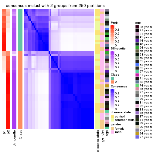
consensus_heatmap(res, k = 3)
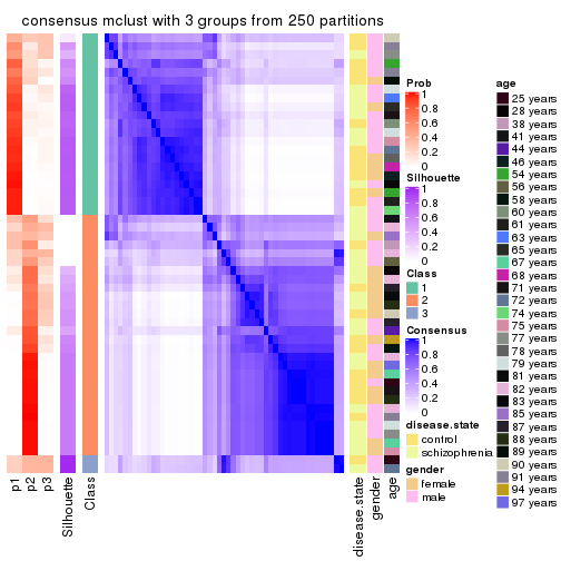
consensus_heatmap(res, k = 4)
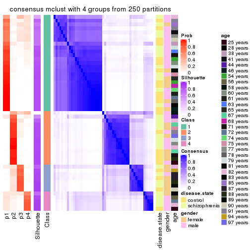
consensus_heatmap(res, k = 5)
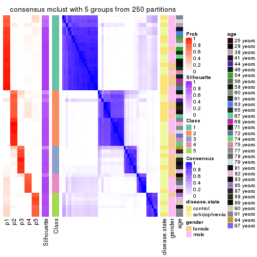
consensus_heatmap(res, k = 6)
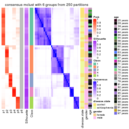
Heatmaps for the membership of samples in all partitions to see how consistent they are:
membership_heatmap(res, k = 2)
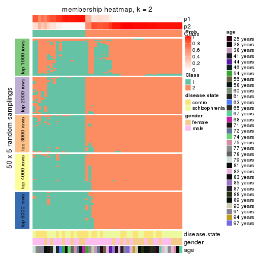
membership_heatmap(res, k = 3)
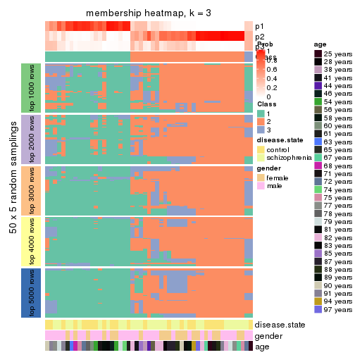
membership_heatmap(res, k = 4)
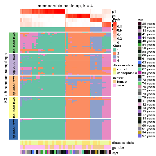
membership_heatmap(res, k = 5)
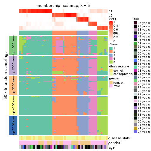
membership_heatmap(res, k = 6)
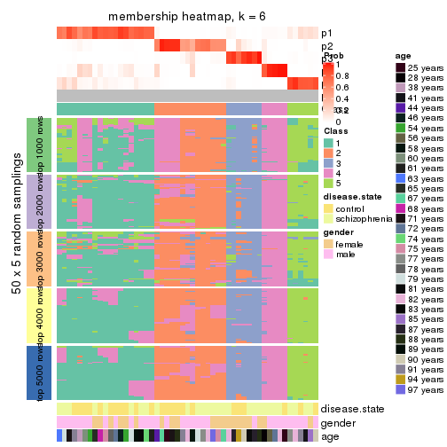
As soon as we have had the classes for columns, we can look for signatures which are significantly different between classes which can be candidate marks for certain classes. Following are the heatmaps for signatures.
Signature heatmaps where rows are scaled:
get_signatures(res, k = 2)

get_signatures(res, k = 3)
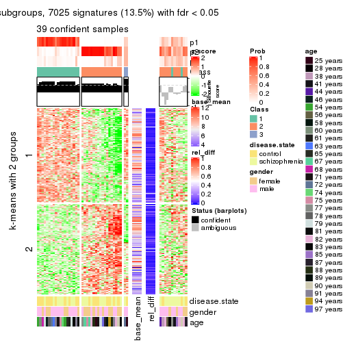
get_signatures(res, k = 4)
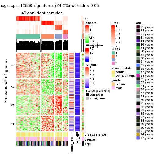
get_signatures(res, k = 5)
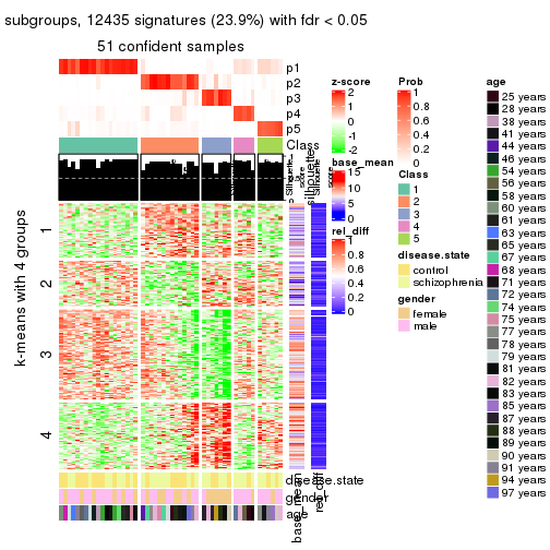
get_signatures(res, k = 6)
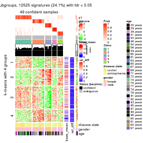
Signature heatmaps where rows are not scaled:
get_signatures(res, k = 2, scale_rows = FALSE)
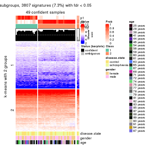
get_signatures(res, k = 3, scale_rows = FALSE)
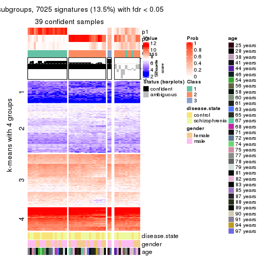
get_signatures(res, k = 4, scale_rows = FALSE)
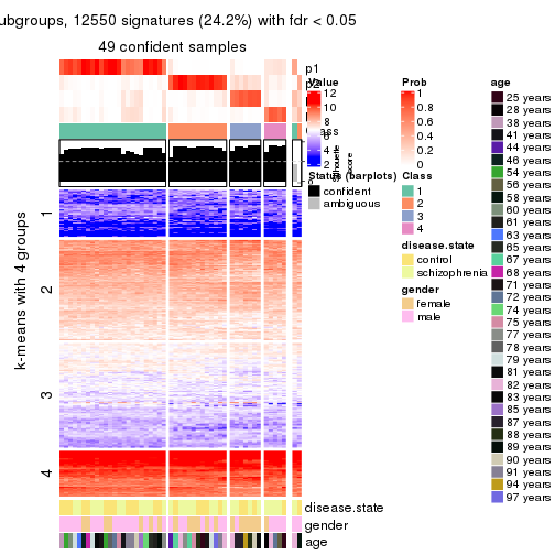
get_signatures(res, k = 5, scale_rows = FALSE)
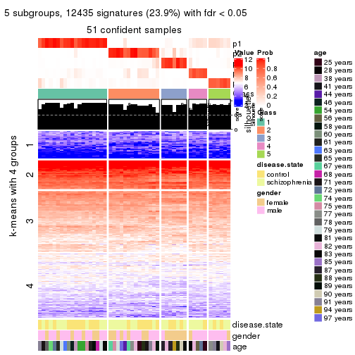
get_signatures(res, k = 6, scale_rows = FALSE)
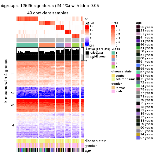
Compare the overlap of signatures from different k:
compare_signatures(res)
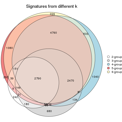
get_signature() returns a data frame invisibly. TO get the list of signatures, the function
call should be assigned to a variable explicitly. In following code, if plot argument is set
to FALSE, no heatmap is plotted while only the differential analysis is performed.
# code only for demonstration
tb = get_signature(res, k = ..., plot = FALSE)
An example of the output of tb is:
#>   which_row         fdr    mean_1    mean_2 scaled_mean_1 scaled_mean_2 km
#> 1        38 0.042760348  8.373488  9.131774    -0.5533452     0.5164555  1
#> 2        40 0.018707592  7.106213  8.469186    -0.6173731     0.5762149  1
#> 3        55 0.019134737 10.221463 11.207825    -0.6159697     0.5749050  1
#> 4        59 0.006059896  5.921854  7.869574    -0.6899429     0.6439467  1
#> 5        60 0.018055526  8.928898 10.211722    -0.6204761     0.5791110  1
#> 6        98 0.009384629 15.714769 14.887706     0.6635654    -0.6193277  2
...
The columns in tb are:
which_row: row indices corresponding to the input matrix.fdr: FDR for the differential test. mean_x: The mean value in group x.scaled_mean_x: The mean value in group x after rows are scaled.km: Row groups if k-means clustering is applied to rows.UMAP plot which shows how samples are separated.
dimension_reduction(res, k = 2, method = "UMAP")
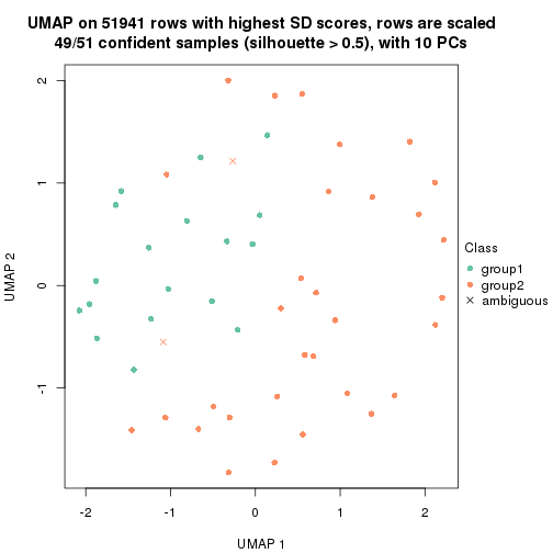
dimension_reduction(res, k = 3, method = "UMAP")
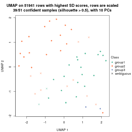
dimension_reduction(res, k = 4, method = "UMAP")
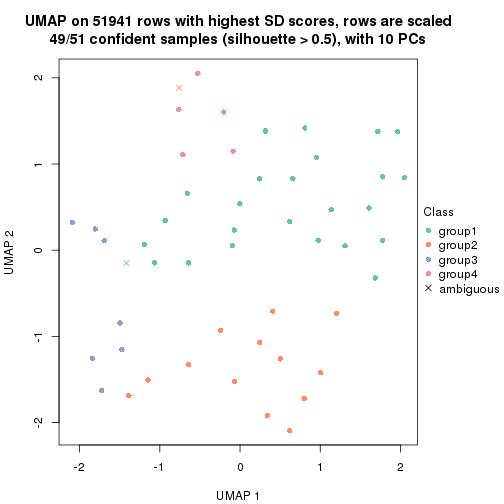
dimension_reduction(res, k = 5, method = "UMAP")
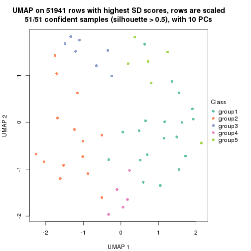
dimension_reduction(res, k = 6, method = "UMAP")
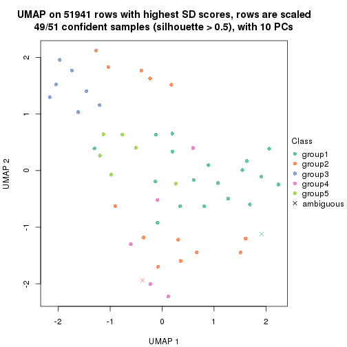
Following heatmap shows how subgroups are split when increasing k:
collect_classes(res)
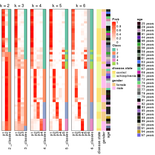
Test correlation between subgroups and known annotations. If the known annotation is numeric, one-way ANOVA test is applied, and if the known annotation is discrete, chi-squared contingency table test is applied.
test_to_known_factors(res)
#>            n disease.state(p) gender(p) age(p) k
#> SD:mclust 49            0.398    0.6096  0.256 2
#> SD:mclust 39            0.715    0.1602  0.688 3
#> SD:mclust 49            0.510    0.0413  0.523 4
#> SD:mclust 51            0.574    0.0625  0.543 5
#> SD:mclust 49            0.631    0.0675  0.510 6
If matrix rows can be associated to genes, consider to use functional_enrichment(res,
...) to perform function enrichment for the signature genes. See this vignette for more detailed explanations.
The object with results only for a single top-value method and a single partition method can be extracted as:
res = res_list["SD", "NMF"]
# you can also extract it by
# res = res_list["SD:NMF"]
A summary of res and all the functions that can be applied to it:
res
#> A 'ConsensusPartition' object with k = 2, 3, 4, 5, 6.
#>   On a matrix with 51941 rows and 51 columns.
#>   Top rows (1000, 2000, 3000, 4000, 5000) are extracted by 'SD' method.
#>   Subgroups are detected by 'NMF' method.
#>   Performed in total 1250 partitions by row resampling.
#>   Best k for subgroups seems to be 2.
#>
#> Following methods can be applied to this 'ConsensusPartition' object:
#>  [1] "cola_report"             "collect_classes"         "collect_plots"
#>  [4] "collect_stats"           "colnames"                "compare_signatures"
#>  [7] "consensus_heatmap"       "dimension_reduction"     "functional_enrichment"
#> [10] "get_anno_col"            "get_anno"                "get_classes"
#> [13] "get_consensus"           "get_matrix"              "get_membership"
#> [16] "get_param"               "get_signatures"          "get_stats"
#> [19] "is_best_k"               "is_stable_k"             "membership_heatmap"
#> [22] "ncol"                    "nrow"                    "plot_ecdf"
#> [25] "rownames"                "select_partition_number" "show"
#> [28] "suggest_best_k"          "test_to_known_factors"
collect_plots() function collects all the plots made from res for all k (number of partitions)
into one single page to provide an easy and fast comparison between different k.
collect_plots(res)
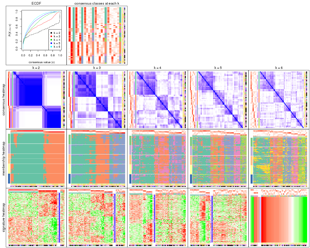
The plots are:
k and the heatmap of
predicted classes for each k.k.k.k.All the plots in panels can be made by individual functions and they are plotted later in this section.
select_partition_number() produces several plots showing different
statistics for choosing “optimized” k. There are following statistics:
k;k, the area increased is defined as \(A_k - A_{k-1}\).The detailed explanations of these statistics can be found in the cola vignette.
Generally speaking, lower PAC score, higher mean silhouette score or higher
concordance corresponds to better partition. Rand index and Jaccard index
measure how similar the current partition is compared to partition with k-1.
If they are too similar, we won't accept k is better than k-1.
select_partition_number(res)
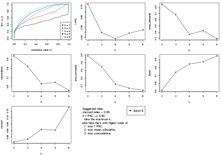
The numeric values for all these statistics can be obtained by get_stats().
get_stats(res)
#>   k 1-PAC mean_silhouette concordance area_increased  Rand Jaccard
#> 2 2 0.725           0.845       0.938         0.4893 0.514   0.514
#> 3 3 0.449           0.681       0.824         0.3486 0.740   0.534
#> 4 4 0.389           0.367       0.633         0.1241 0.845   0.608
#> 5 5 0.442           0.427       0.648         0.0702 0.874   0.604
#> 6 6 0.473           0.300       0.561         0.0430 0.947   0.776
suggest_best_k() suggests the best \(k\) based on these statistics. The rules are as follows:
suggest_best_k(res)
#> [1] 2
Following shows the table of the partitions (You need to click the show/hide
code output link to see it). The membership matrix (columns with name p*)
is inferred by
clue::cl_consensus()
function with the SE method. Basically the value in the membership matrix
represents the probability to belong to a certain group. The finall class
label for an item is determined with the group with highest probability it
belongs to.
In get_classes() function, the entropy is calculated from the membership
matrix and the silhouette score is calculated from the consensus matrix.
cbind(get_classes(res, k = 2), get_membership(res, k = 2))
#>           class entropy silhouette    p1    p2
#> GSM439800     2  0.9909     0.2066 0.444 0.556
#> GSM439790     1  0.0938     0.9239 0.988 0.012
#> GSM439827     2  0.0000     0.9273 0.000 1.000
#> GSM439811     2  0.0000     0.9273 0.000 1.000
#> GSM439795     2  0.0000     0.9273 0.000 1.000
#> GSM439805     2  0.9754     0.2751 0.408 0.592
#> GSM439781     1  0.7815     0.6906 0.768 0.232
#> GSM439807     2  0.6438     0.7716 0.164 0.836
#> GSM439820     2  0.0000     0.9273 0.000 1.000
#> GSM439784     1  0.0938     0.9242 0.988 0.012
#> GSM439824     1  0.9998    -0.0215 0.508 0.492
#> GSM439794     1  0.9248     0.4585 0.660 0.340
#> GSM439809     1  0.0000     0.9292 1.000 0.000
#> GSM439785     1  0.0938     0.9229 0.988 0.012
#> GSM439803     1  0.0000     0.9292 1.000 0.000
#> GSM439778     1  0.0000     0.9292 1.000 0.000
#> GSM439791     1  0.0000     0.9292 1.000 0.000
#> GSM439786     1  0.2778     0.8968 0.952 0.048
#> GSM439828     2  0.0376     0.9256 0.004 0.996
#> GSM439806     1  0.0000     0.9292 1.000 0.000
#> GSM439815     1  0.0000     0.9292 1.000 0.000
#> GSM439817     2  0.0000     0.9273 0.000 1.000
#> GSM439796     1  0.8661     0.5695 0.712 0.288
#> GSM439798     1  0.6343     0.7845 0.840 0.160
#> GSM439821     2  0.0000     0.9273 0.000 1.000
#> GSM439823     2  0.0376     0.9256 0.004 0.996
#> GSM439813     1  0.0000     0.9292 1.000 0.000
#> GSM439801     2  0.0376     0.9254 0.004 0.996
#> GSM439810     1  0.0000     0.9292 1.000 0.000
#> GSM439783     1  0.0000     0.9292 1.000 0.000
#> GSM439826     2  0.4562     0.8523 0.096 0.904
#> GSM439812     1  0.0000     0.9292 1.000 0.000
#> GSM439818     2  0.0000     0.9273 0.000 1.000
#> GSM439792     1  0.0000     0.9292 1.000 0.000
#> GSM439802     1  0.8499     0.6167 0.724 0.276
#> GSM439825     2  0.0000     0.9273 0.000 1.000
#> GSM439780     1  0.0000     0.9292 1.000 0.000
#> GSM439787     2  0.0000     0.9273 0.000 1.000
#> GSM439808     2  0.0000     0.9273 0.000 1.000
#> GSM439804     1  0.0000     0.9292 1.000 0.000
#> GSM439822     2  0.5629     0.8144 0.132 0.868
#> GSM439816     1  0.0000     0.9292 1.000 0.000
#> GSM439789     1  0.0000     0.9292 1.000 0.000
#> GSM439799     2  0.0000     0.9273 0.000 1.000
#> GSM439814     1  0.0000     0.9292 1.000 0.000
#> GSM439782     1  0.0000     0.9292 1.000 0.000
#> GSM439779     1  0.0000     0.9292 1.000 0.000
#> GSM439793     1  0.1184     0.9218 0.984 0.016
#> GSM439788     1  0.0376     0.9277 0.996 0.004
#> GSM439797     1  0.0938     0.9242 0.988 0.012
#> GSM439819     2  0.0000     0.9273 0.000 1.000
cbind(get_classes(res, k = 3), get_membership(res, k = 3))
#>           class entropy silhouette    p1    p2    p3
#> GSM439800     3   0.834      0.471 0.144 0.236 0.620
#> GSM439790     3   0.613      0.305 0.400 0.000 0.600
#> GSM439827     2   0.478      0.818 0.016 0.820 0.164
#> GSM439811     2   0.463      0.796 0.004 0.808 0.188
#> GSM439795     3   0.394      0.588 0.000 0.156 0.844
#> GSM439805     3   0.165      0.679 0.004 0.036 0.960
#> GSM439781     3   0.145      0.696 0.024 0.008 0.968
#> GSM439807     3   0.271      0.649 0.000 0.088 0.912
#> GSM439820     2   0.543      0.663 0.000 0.716 0.284
#> GSM439784     1   0.506      0.764 0.816 0.028 0.156
#> GSM439824     1   0.627      0.209 0.544 0.456 0.000
#> GSM439794     1   0.663      0.519 0.644 0.336 0.020
#> GSM439809     1   0.435      0.770 0.836 0.008 0.156
#> GSM439785     1   0.277      0.779 0.916 0.080 0.004
#> GSM439803     1   0.416      0.744 0.848 0.144 0.008
#> GSM439778     1   0.435      0.743 0.816 0.000 0.184
#> GSM439791     1   0.312      0.799 0.908 0.012 0.080
#> GSM439786     3   0.585      0.631 0.188 0.040 0.772
#> GSM439828     2   0.220      0.830 0.056 0.940 0.004
#> GSM439806     1   0.382      0.776 0.852 0.000 0.148
#> GSM439815     1   0.603      0.765 0.776 0.060 0.164
#> GSM439817     2   0.203      0.848 0.032 0.952 0.016
#> GSM439796     1   0.620      0.497 0.656 0.336 0.008
#> GSM439798     3   0.429      0.691 0.104 0.032 0.864
#> GSM439821     2   0.369      0.826 0.000 0.860 0.140
#> GSM439823     2   0.195      0.837 0.040 0.952 0.008
#> GSM439813     1   0.435      0.742 0.816 0.000 0.184
#> GSM439801     3   0.522      0.495 0.000 0.260 0.740
#> GSM439810     1   0.186      0.800 0.948 0.000 0.052
#> GSM439783     1   0.175      0.800 0.960 0.012 0.028
#> GSM439826     2   0.536      0.683 0.196 0.784 0.020
#> GSM439812     1   0.345      0.798 0.888 0.008 0.104
#> GSM439818     2   0.236      0.853 0.000 0.928 0.072
#> GSM439792     1   0.394      0.774 0.844 0.000 0.156
#> GSM439802     3   0.113      0.695 0.020 0.004 0.976
#> GSM439825     2   0.196      0.853 0.000 0.944 0.056
#> GSM439780     3   0.613      0.325 0.400 0.000 0.600
#> GSM439787     3   0.497      0.497 0.000 0.236 0.764
#> GSM439808     3   0.613      0.105 0.000 0.400 0.600
#> GSM439804     1   0.497      0.702 0.800 0.188 0.012
#> GSM439822     2   0.238      0.830 0.056 0.936 0.008
#> GSM439816     1   0.429      0.710 0.820 0.180 0.000
#> GSM439789     1   0.116      0.793 0.972 0.028 0.000
#> GSM439799     2   0.382      0.822 0.000 0.852 0.148
#> GSM439814     1   0.103      0.794 0.976 0.024 0.000
#> GSM439782     1   0.502      0.666 0.760 0.000 0.240
#> GSM439779     1   0.348      0.782 0.872 0.000 0.128
#> GSM439793     3   0.533      0.589 0.248 0.004 0.748
#> GSM439788     3   0.653      0.306 0.404 0.008 0.588
#> GSM439797     1   0.295      0.786 0.920 0.060 0.020
#> GSM439819     2   0.355      0.829 0.000 0.868 0.132
cbind(get_classes(res, k = 4), get_membership(res, k = 4))
#>           class entropy silhouette    p1    p2    p3    p4
#> GSM439800     3   0.852    0.00425 0.064 0.156 0.476 0.304
#> GSM439790     1   0.660    0.15791 0.488 0.000 0.432 0.080
#> GSM439827     2   0.892    0.30480 0.072 0.412 0.192 0.324
#> GSM439811     2   0.853    0.23375 0.028 0.392 0.264 0.316
#> GSM439795     3   0.338    0.53419 0.000 0.076 0.872 0.052
#> GSM439805     3   0.221    0.56211 0.028 0.000 0.928 0.044
#> GSM439781     3   0.689    0.50586 0.100 0.028 0.640 0.232
#> GSM439807     3   0.119    0.57308 0.004 0.024 0.968 0.004
#> GSM439820     2   0.771    0.23466 0.000 0.440 0.316 0.244
#> GSM439784     1   0.804    0.09239 0.440 0.032 0.140 0.388
#> GSM439824     2   0.700    0.02094 0.368 0.508 0.000 0.124
#> GSM439794     4   0.894    0.31904 0.224 0.352 0.060 0.364
#> GSM439809     1   0.327    0.63835 0.884 0.004 0.060 0.052
#> GSM439785     1   0.468    0.57573 0.772 0.044 0.000 0.184
#> GSM439803     1   0.836   -0.21786 0.412 0.208 0.028 0.352
#> GSM439778     1   0.499    0.57525 0.772 0.000 0.096 0.132
#> GSM439791     1   0.198    0.64415 0.940 0.004 0.016 0.040
#> GSM439786     4   0.781   -0.30426 0.252 0.000 0.372 0.376
#> GSM439828     2   0.499    0.49727 0.028 0.744 0.008 0.220
#> GSM439806     1   0.410    0.61335 0.816 0.000 0.036 0.148
#> GSM439815     1   0.820    0.26006 0.504 0.056 0.132 0.308
#> GSM439817     2   0.436    0.51288 0.016 0.780 0.004 0.200
#> GSM439796     2   0.810   -0.43173 0.188 0.432 0.020 0.360
#> GSM439798     3   0.744    0.34507 0.148 0.004 0.444 0.404
#> GSM439821     2   0.642    0.46395 0.000 0.640 0.132 0.228
#> GSM439823     2   0.490    0.29409 0.008 0.688 0.004 0.300
#> GSM439813     1   0.506    0.58010 0.768 0.000 0.108 0.124
#> GSM439801     3   0.705    0.20620 0.000 0.124 0.484 0.392
#> GSM439810     1   0.340    0.63631 0.888 0.040 0.028 0.044
#> GSM439783     1   0.635    0.57643 0.728 0.092 0.072 0.108
#> GSM439826     2   0.504    0.40165 0.072 0.800 0.028 0.100
#> GSM439812     1   0.517    0.61867 0.788 0.044 0.128 0.040
#> GSM439818     2   0.442    0.50219 0.000 0.788 0.176 0.036
#> GSM439792     1   0.535    0.59245 0.756 0.008 0.156 0.080
#> GSM439802     3   0.396    0.51065 0.052 0.000 0.836 0.112
#> GSM439825     2   0.376    0.51592 0.000 0.828 0.152 0.020
#> GSM439780     3   0.667    0.18422 0.320 0.000 0.572 0.108
#> GSM439787     3   0.545    0.50798 0.000 0.080 0.724 0.196
#> GSM439808     3   0.693    0.28588 0.000 0.228 0.588 0.184
#> GSM439804     4   0.853    0.31275 0.292 0.332 0.024 0.352
#> GSM439822     2   0.252    0.41930 0.004 0.904 0.004 0.088
#> GSM439816     1   0.662    0.27287 0.576 0.320 0.000 0.104
#> GSM439789     1   0.417    0.59890 0.828 0.080 0.000 0.092
#> GSM439799     4   0.697   -0.13250 0.000 0.428 0.112 0.460
#> GSM439814     1   0.383    0.60547 0.848 0.084 0.000 0.068
#> GSM439782     1   0.622    0.48683 0.668 0.000 0.144 0.188
#> GSM439779     1   0.202    0.64519 0.936 0.000 0.040 0.024
#> GSM439793     3   0.775    0.18882 0.360 0.000 0.404 0.236
#> GSM439788     1   0.731    0.25936 0.524 0.000 0.284 0.192
#> GSM439797     1   0.549    0.42108 0.624 0.028 0.000 0.348
#> GSM439819     2   0.622    0.49108 0.000 0.648 0.104 0.248
cbind(get_classes(res, k = 5), get_membership(res, k = 5))
#>           class entropy silhouette    p1    p2    p3    p4    p5
#> GSM439800     3   0.582     0.4961 0.052 0.052 0.696 0.184 0.016
#> GSM439790     1   0.673     0.1896 0.496 0.000 0.360 0.044 0.100
#> GSM439827     2   0.508     0.4118 0.060 0.692 0.012 0.000 0.236
#> GSM439811     2   0.584     0.4059 0.044 0.640 0.060 0.000 0.256
#> GSM439795     3   0.295     0.6355 0.000 0.016 0.884 0.052 0.048
#> GSM439805     3   0.344     0.6437 0.032 0.008 0.856 0.012 0.092
#> GSM439781     3   0.721     0.1648 0.108 0.072 0.412 0.000 0.408
#> GSM439807     3   0.348     0.6453 0.016 0.040 0.848 0.000 0.096
#> GSM439820     2   0.703     0.3378 0.004 0.480 0.192 0.020 0.304
#> GSM439784     5   0.581     0.4360 0.244 0.100 0.012 0.004 0.640
#> GSM439824     2   0.524     0.3088 0.260 0.664 0.000 0.068 0.008
#> GSM439794     4   0.491     0.6807 0.132 0.052 0.056 0.760 0.000
#> GSM439809     1   0.353     0.5762 0.856 0.024 0.012 0.020 0.088
#> GSM439785     1   0.723     0.1885 0.500 0.056 0.000 0.276 0.168
#> GSM439803     4   0.478     0.4818 0.296 0.008 0.028 0.668 0.000
#> GSM439778     1   0.451     0.5706 0.776 0.000 0.076 0.132 0.016
#> GSM439791     1   0.276     0.5961 0.888 0.008 0.000 0.072 0.032
#> GSM439786     5   0.661     0.4408 0.220 0.000 0.048 0.140 0.592
#> GSM439828     2   0.590     0.4629 0.000 0.596 0.000 0.168 0.236
#> GSM439806     1   0.481     0.4076 0.716 0.044 0.008 0.004 0.228
#> GSM439815     1   0.671     0.1669 0.456 0.000 0.104 0.404 0.036
#> GSM439817     2   0.617     0.4776 0.000 0.600 0.012 0.168 0.220
#> GSM439796     4   0.356     0.6985 0.100 0.024 0.032 0.844 0.000
#> GSM439798     5   0.377     0.4555 0.068 0.000 0.076 0.020 0.836
#> GSM439821     2   0.824     0.2943 0.000 0.360 0.180 0.308 0.152
#> GSM439823     4   0.579     0.2964 0.000 0.184 0.000 0.616 0.200
#> GSM439813     1   0.516     0.5663 0.728 0.000 0.132 0.120 0.020
#> GSM439801     5   0.742     0.0170 0.000 0.028 0.316 0.304 0.352
#> GSM439810     1   0.471     0.4826 0.688 0.280 0.008 0.012 0.012
#> GSM439783     1   0.744     0.4457 0.532 0.232 0.160 0.064 0.012
#> GSM439826     2   0.393     0.4715 0.020 0.804 0.016 0.156 0.004
#> GSM439812     1   0.678     0.4937 0.616 0.168 0.160 0.028 0.028
#> GSM439818     2   0.651     0.4276 0.000 0.556 0.244 0.184 0.016
#> GSM439792     1   0.610     0.5003 0.648 0.152 0.172 0.004 0.024
#> GSM439802     3   0.435     0.6008 0.076 0.000 0.800 0.028 0.096
#> GSM439825     2   0.628     0.4455 0.000 0.596 0.192 0.196 0.016
#> GSM439780     3   0.554     0.2838 0.316 0.000 0.616 0.028 0.040
#> GSM439787     3   0.535     0.5107 0.000 0.060 0.628 0.008 0.304
#> GSM439808     3   0.563     0.5225 0.000 0.124 0.672 0.016 0.188
#> GSM439804     4   0.401     0.6694 0.160 0.008 0.032 0.796 0.004
#> GSM439822     2   0.571     0.2933 0.000 0.548 0.060 0.380 0.012
#> GSM439816     2   0.571    -0.0664 0.400 0.528 0.000 0.064 0.008
#> GSM439789     1   0.455     0.5857 0.768 0.068 0.004 0.152 0.008
#> GSM439799     4   0.494     0.5183 0.000 0.076 0.068 0.768 0.088
#> GSM439814     1   0.496     0.5495 0.728 0.192 0.000 0.056 0.024
#> GSM439782     1   0.557     0.5245 0.684 0.000 0.100 0.192 0.024
#> GSM439779     1   0.229     0.6035 0.924 0.016 0.032 0.012 0.016
#> GSM439793     5   0.600     0.3924 0.284 0.012 0.112 0.000 0.592
#> GSM439788     1   0.633    -0.1084 0.484 0.004 0.080 0.020 0.412
#> GSM439797     5   0.753     0.2399 0.304 0.044 0.000 0.248 0.404
#> GSM439819     2   0.741     0.3229 0.000 0.416 0.096 0.104 0.384
cbind(get_classes(res, k = 6), get_membership(res, k = 6))
#>           class entropy silhouette    p1    p2    p3    p4    p5    p6
#> GSM439800     3   0.674     0.2614 0.048 0.044 0.576 0.104 0.008 0.220
#> GSM439790     1   0.740     0.1741 0.432 0.004 0.332 0.036 0.104 0.092
#> GSM439827     2   0.546     0.4141 0.032 0.640 0.008 0.000 0.240 0.080
#> GSM439811     2   0.620     0.3583 0.016 0.552 0.032 0.000 0.284 0.116
#> GSM439795     3   0.228     0.4524 0.000 0.008 0.908 0.024 0.008 0.052
#> GSM439805     3   0.356     0.4634 0.052 0.000 0.840 0.008 0.048 0.052
#> GSM439781     5   0.722     0.0442 0.104 0.028 0.364 0.000 0.408 0.096
#> GSM439807     3   0.486     0.1007 0.028 0.004 0.572 0.004 0.008 0.384
#> GSM439820     2   0.773     0.1525 0.008 0.364 0.100 0.020 0.172 0.336
#> GSM439784     5   0.650     0.3477 0.252 0.060 0.036 0.000 0.568 0.084
#> GSM439824     2   0.567     0.2572 0.272 0.600 0.000 0.036 0.004 0.088
#> GSM439794     4   0.632     0.5631 0.188 0.068 0.048 0.628 0.004 0.064
#> GSM439809     1   0.542     0.4867 0.692 0.024 0.016 0.020 0.060 0.188
#> GSM439785     1   0.753     0.1391 0.432 0.056 0.000 0.260 0.200 0.052
#> GSM439803     4   0.545     0.4902 0.264 0.024 0.012 0.644 0.024 0.032
#> GSM439778     1   0.606     0.4492 0.680 0.004 0.084 0.084 0.076 0.072
#> GSM439791     1   0.412     0.5357 0.800 0.008 0.000 0.064 0.044 0.084
#> GSM439786     5   0.661     0.3841 0.128 0.000 0.064 0.152 0.604 0.052
#> GSM439828     2   0.589     0.4188 0.008 0.608 0.000 0.060 0.244 0.080
#> GSM439806     1   0.660     0.4034 0.580 0.080 0.012 0.004 0.172 0.152
#> GSM439815     6   0.774    -0.1475 0.252 0.020 0.076 0.288 0.008 0.356
#> GSM439817     2   0.681     0.4189 0.016 0.568 0.004 0.112 0.176 0.124
#> GSM439796     4   0.402     0.6463 0.076 0.080 0.008 0.808 0.004 0.024
#> GSM439798     5   0.391     0.4448 0.064 0.000 0.068 0.020 0.820 0.028
#> GSM439821     2   0.872     0.2603 0.000 0.316 0.144 0.212 0.144 0.184
#> GSM439823     4   0.698     0.2341 0.004 0.256 0.004 0.476 0.188 0.072
#> GSM439813     1   0.633     0.0862 0.484 0.004 0.080 0.060 0.004 0.368
#> GSM439801     3   0.784     0.0680 0.008 0.016 0.360 0.244 0.268 0.104
#> GSM439810     1   0.608     0.3831 0.556 0.248 0.012 0.004 0.008 0.172
#> GSM439783     1   0.707     0.4139 0.580 0.132 0.148 0.048 0.012 0.080
#> GSM439826     2   0.315     0.4707 0.028 0.860 0.000 0.064 0.004 0.044
#> GSM439812     1   0.693     0.0521 0.400 0.128 0.060 0.008 0.008 0.396
#> GSM439818     2   0.669     0.3815 0.000 0.544 0.216 0.104 0.008 0.128
#> GSM439792     1   0.571     0.4824 0.696 0.064 0.132 0.004 0.040 0.064
#> GSM439802     3   0.423     0.4260 0.040 0.004 0.800 0.044 0.016 0.096
#> GSM439825     2   0.671     0.3906 0.004 0.544 0.196 0.068 0.008 0.180
#> GSM439780     3   0.682     0.0373 0.352 0.004 0.392 0.016 0.016 0.220
#> GSM439787     3   0.502     0.3210 0.000 0.004 0.652 0.000 0.208 0.136
#> GSM439808     6   0.677    -0.3513 0.004 0.060 0.396 0.004 0.132 0.404
#> GSM439804     4   0.443     0.6236 0.100 0.044 0.008 0.788 0.012 0.048
#> GSM439822     2   0.521     0.3446 0.000 0.636 0.028 0.260 0.000 0.076
#> GSM439816     2   0.568    -0.0889 0.416 0.484 0.004 0.024 0.000 0.072
#> GSM439789     1   0.443     0.5139 0.784 0.052 0.008 0.092 0.004 0.060
#> GSM439799     4   0.407     0.5559 0.000 0.052 0.032 0.816 0.052 0.048
#> GSM439814     1   0.592     0.3246 0.560 0.136 0.000 0.032 0.000 0.272
#> GSM439782     1   0.626     0.4393 0.648 0.004 0.056 0.152 0.060 0.080
#> GSM439779     1   0.252     0.5401 0.888 0.000 0.008 0.008 0.016 0.080
#> GSM439793     5   0.667     0.3481 0.256 0.004 0.104 0.004 0.532 0.100
#> GSM439788     1   0.652    -0.0338 0.456 0.004 0.080 0.028 0.396 0.036
#> GSM439797     5   0.662     0.1618 0.212 0.012 0.008 0.240 0.508 0.020
#> GSM439819     5   0.776    -0.3355 0.000 0.336 0.052 0.068 0.348 0.196
Heatmaps for the consensus matrix. It visualizes the probability of two samples to be in a same group.
consensus_heatmap(res, k = 2)
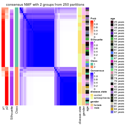
consensus_heatmap(res, k = 3)
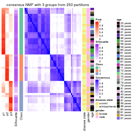
consensus_heatmap(res, k = 4)
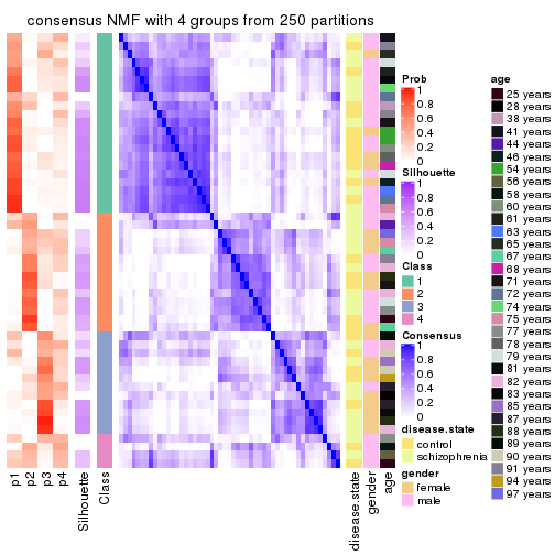
consensus_heatmap(res, k = 5)
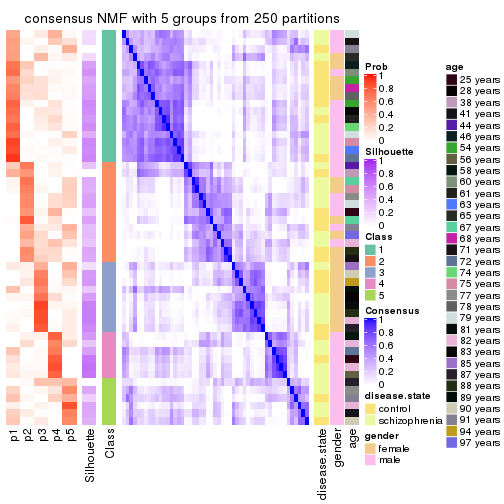
consensus_heatmap(res, k = 6)
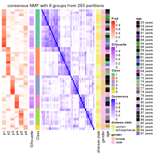
Heatmaps for the membership of samples in all partitions to see how consistent they are:
membership_heatmap(res, k = 2)
membership_heatmap(res, k = 3)
membership_heatmap(res, k = 4)
membership_heatmap(res, k = 5)
membership_heatmap(res, k = 6)
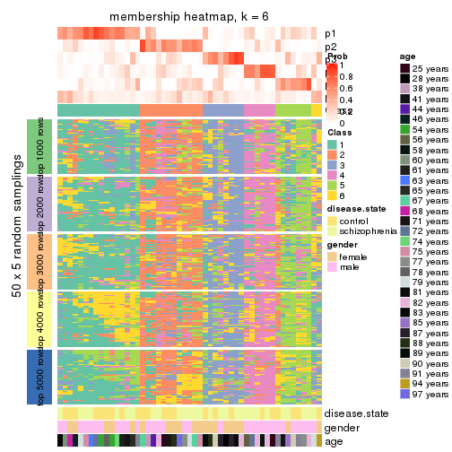
As soon as we have had the classes for columns, we can look for signatures which are significantly different between classes which can be candidate marks for certain classes. Following are the heatmaps for signatures.
Signature heatmaps where rows are scaled:
get_signatures(res, k = 2)
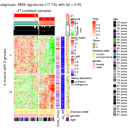
get_signatures(res, k = 3)
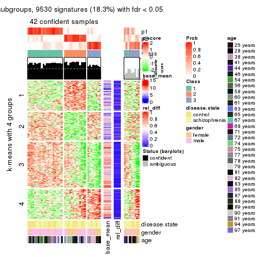
get_signatures(res, k = 4)
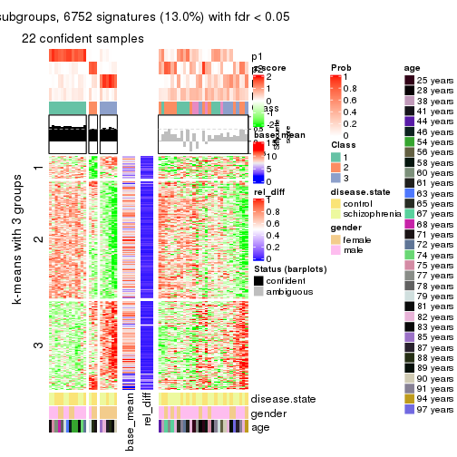
get_signatures(res, k = 5)
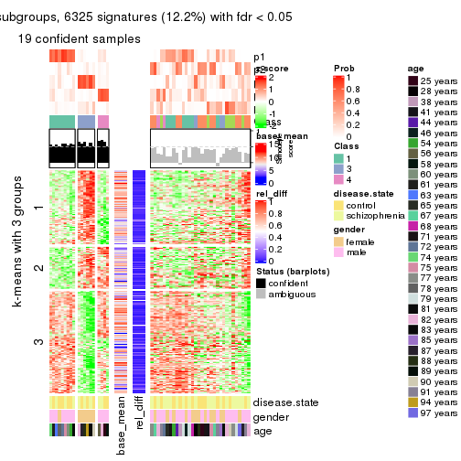
get_signatures(res, k = 6)
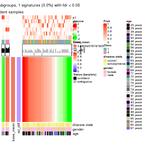
Signature heatmaps where rows are not scaled:
get_signatures(res, k = 2, scale_rows = FALSE)
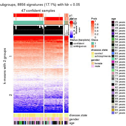
get_signatures(res, k = 3, scale_rows = FALSE)
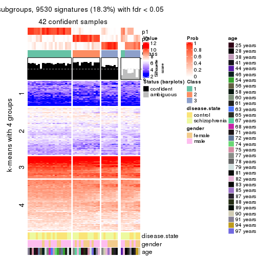
get_signatures(res, k = 4, scale_rows = FALSE)
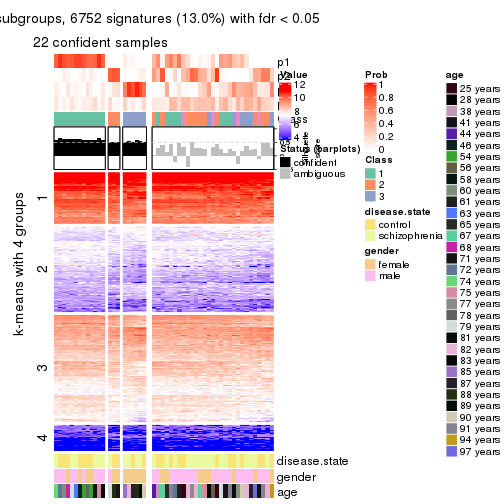
get_signatures(res, k = 5, scale_rows = FALSE)
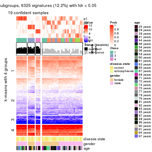
get_signatures(res, k = 6, scale_rows = FALSE)
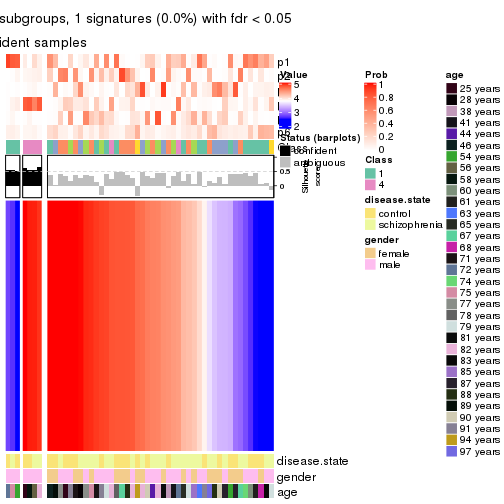
Compare the overlap of signatures from different k:
compare_signatures(res)
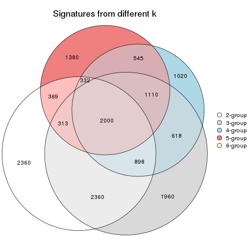
get_signature() returns a data frame invisibly. TO get the list of signatures, the function
call should be assigned to a variable explicitly. In following code, if plot argument is set
to FALSE, no heatmap is plotted while only the differential analysis is performed.
# code only for demonstration
tb = get_signature(res, k = ..., plot = FALSE)
An example of the output of tb is:
#>   which_row         fdr    mean_1    mean_2 scaled_mean_1 scaled_mean_2 km
#> 1        38 0.042760348  8.373488  9.131774    -0.5533452     0.5164555  1
#> 2        40 0.018707592  7.106213  8.469186    -0.6173731     0.5762149  1
#> 3        55 0.019134737 10.221463 11.207825    -0.6159697     0.5749050  1
#> 4        59 0.006059896  5.921854  7.869574    -0.6899429     0.6439467  1
#> 5        60 0.018055526  8.928898 10.211722    -0.6204761     0.5791110  1
#> 6        98 0.009384629 15.714769 14.887706     0.6635654    -0.6193277  2
...
The columns in tb are:
which_row: row indices corresponding to the input matrix.fdr: FDR for the differential test. mean_x: The mean value in group x.scaled_mean_x: The mean value in group x after rows are scaled.km: Row groups if k-means clustering is applied to rows.UMAP plot which shows how samples are separated.
dimension_reduction(res, k = 2, method = "UMAP")
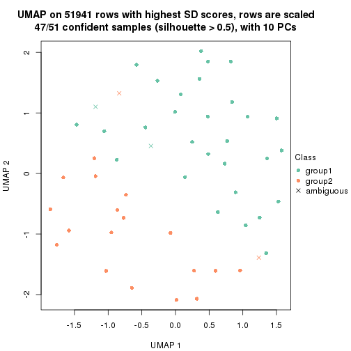
dimension_reduction(res, k = 3, method = "UMAP")
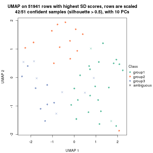
dimension_reduction(res, k = 4, method = "UMAP")
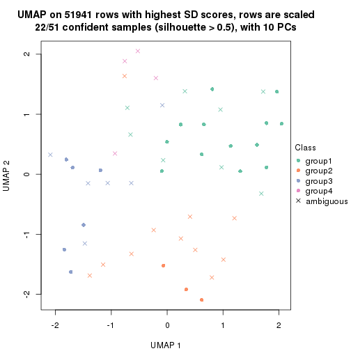
dimension_reduction(res, k = 5, method = "UMAP")
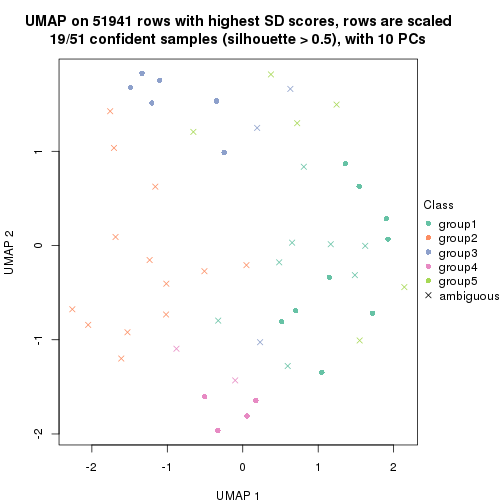
dimension_reduction(res, k = 6, method = "UMAP")

Following heatmap shows how subgroups are split when increasing k:
collect_classes(res)
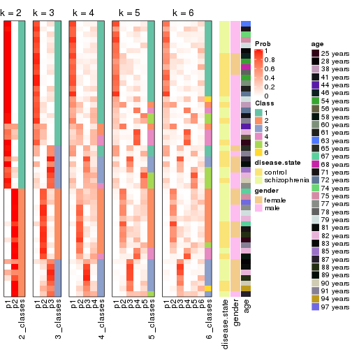
Test correlation between subgroups and known annotations. If the known annotation is numeric, one-way ANOVA test is applied, and if the known annotation is discrete, chi-squared contingency table test is applied.
test_to_known_factors(res)
#>         n disease.state(p) gender(p) age(p) k
#> SD:NMF 47            0.853  0.107650  0.707 2
#> SD:NMF 42            0.415  0.059077  0.509 3
#> SD:NMF 22            0.584  0.017061  0.689 4
#> SD:NMF 19            0.971  0.000506  0.466 5
#> SD:NMF  7            1.000        NA  0.321 6
If matrix rows can be associated to genes, consider to use functional_enrichment(res,
...) to perform function enrichment for the signature genes. See this vignette for more detailed explanations.
The object with results only for a single top-value method and a single partition method can be extracted as:
res = res_list["CV", "hclust"]
# you can also extract it by
# res = res_list["CV:hclust"]
A summary of res and all the functions that can be applied to it:
res
#> A 'ConsensusPartition' object with k = 2, 3, 4, 5, 6.
#>   On a matrix with 51941 rows and 51 columns.
#>   Top rows (1000, 2000, 3000, 4000, 5000) are extracted by 'CV' method.
#>   Subgroups are detected by 'hclust' method.
#>   Performed in total 1250 partitions by row resampling.
#>   Best k for subgroups seems to be 2.
#>
#> Following methods can be applied to this 'ConsensusPartition' object:
#>  [1] "cola_report"             "collect_classes"         "collect_plots"
#>  [4] "collect_stats"           "colnames"                "compare_signatures"
#>  [7] "consensus_heatmap"       "dimension_reduction"     "functional_enrichment"
#> [10] "get_anno_col"            "get_anno"                "get_classes"
#> [13] "get_consensus"           "get_matrix"              "get_membership"
#> [16] "get_param"               "get_signatures"          "get_stats"
#> [19] "is_best_k"               "is_stable_k"             "membership_heatmap"
#> [22] "ncol"                    "nrow"                    "plot_ecdf"
#> [25] "rownames"                "select_partition_number" "show"
#> [28] "suggest_best_k"          "test_to_known_factors"
collect_plots() function collects all the plots made from res for all k (number of partitions)
into one single page to provide an easy and fast comparison between different k.
collect_plots(res)
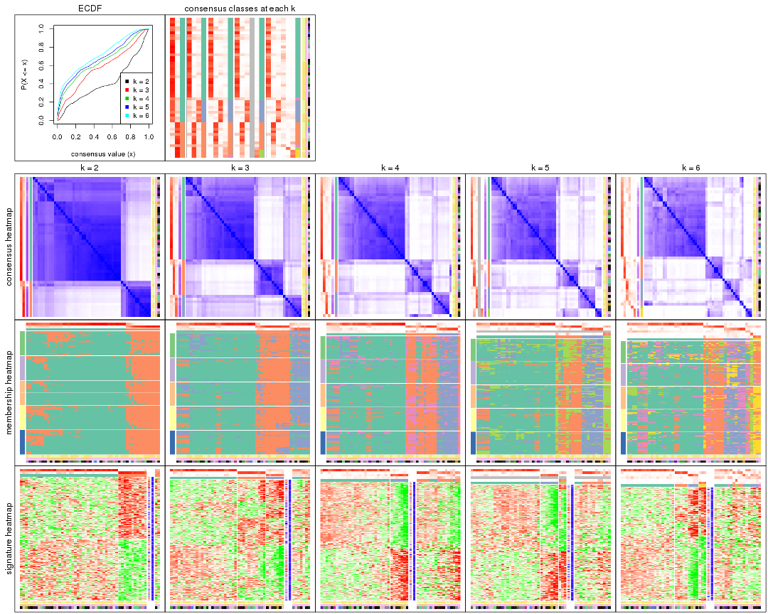
The plots are:
k and the heatmap of
predicted classes for each k.k.k.k.All the plots in panels can be made by individual functions and they are plotted later in this section.
select_partition_number() produces several plots showing different
statistics for choosing “optimized” k. There are following statistics:
k;k, the area increased is defined as \(A_k - A_{k-1}\).The detailed explanations of these statistics can be found in the cola vignette.
Generally speaking, lower PAC score, higher mean silhouette score or higher
concordance corresponds to better partition. Rand index and Jaccard index
measure how similar the current partition is compared to partition with k-1.
If they are too similar, we won't accept k is better than k-1.
select_partition_number(res)
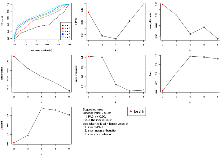
The numeric values for all these statistics can be obtained by get_stats().
get_stats(res)
#>   k 1-PAC mean_silhouette concordance area_increased  Rand Jaccard
#> 2 2 0.412           0.797       0.883         0.4134 0.613   0.613
#> 3 3 0.336           0.694       0.811         0.4038 0.812   0.693
#> 4 4 0.326           0.521       0.763         0.1179 0.991   0.978
#> 5 5 0.384           0.584       0.727         0.0524 0.983   0.959
#> 6 6 0.438           0.475       0.678         0.0582 0.963   0.908
suggest_best_k() suggests the best \(k\) based on these statistics. The rules are as follows:
suggest_best_k(res)
#> [1] 2
Following shows the table of the partitions (You need to click the show/hide
code output link to see it). The membership matrix (columns with name p*)
is inferred by
clue::cl_consensus()
function with the SE method. Basically the value in the membership matrix
represents the probability to belong to a certain group. The finall class
label for an item is determined with the group with highest probability it
belongs to.
In get_classes() function, the entropy is calculated from the membership
matrix and the silhouette score is calculated from the consensus matrix.
cbind(get_classes(res, k = 2), get_membership(res, k = 2))
#>           class entropy silhouette    p1    p2
#> GSM439800     1  0.6801     0.8203 0.820 0.180
#> GSM439790     1  0.3114     0.8723 0.944 0.056
#> GSM439827     2  0.4022     0.8637 0.080 0.920
#> GSM439811     2  0.4022     0.8637 0.080 0.920
#> GSM439795     1  0.6801     0.8149 0.820 0.180
#> GSM439805     1  0.7139     0.8089 0.804 0.196
#> GSM439781     1  0.5294     0.8539 0.880 0.120
#> GSM439807     1  0.6623     0.8224 0.828 0.172
#> GSM439820     2  0.7376     0.7134 0.208 0.792
#> GSM439784     1  0.1414     0.8760 0.980 0.020
#> GSM439824     1  0.8909     0.6152 0.692 0.308
#> GSM439794     1  0.7815     0.7323 0.768 0.232
#> GSM439809     1  0.0672     0.8739 0.992 0.008
#> GSM439785     1  0.7376     0.7453 0.792 0.208
#> GSM439803     1  0.8713     0.6255 0.708 0.292
#> GSM439778     1  0.3114     0.8779 0.944 0.056
#> GSM439791     1  0.2043     0.8781 0.968 0.032
#> GSM439786     1  0.0000     0.8734 1.000 0.000
#> GSM439828     2  0.3431     0.8666 0.064 0.936
#> GSM439806     1  0.0938     0.8757 0.988 0.012
#> GSM439815     1  0.0672     0.8756 0.992 0.008
#> GSM439817     2  0.9710     0.3591 0.400 0.600
#> GSM439796     1  0.8555     0.6467 0.720 0.280
#> GSM439798     1  0.0000     0.8734 1.000 0.000
#> GSM439821     2  0.2043     0.8688 0.032 0.968
#> GSM439823     2  0.5059     0.8376 0.112 0.888
#> GSM439813     1  0.0376     0.8734 0.996 0.004
#> GSM439801     1  0.9044     0.5715 0.680 0.320
#> GSM439810     1  0.3114     0.8723 0.944 0.056
#> GSM439783     1  0.4022     0.8729 0.920 0.080
#> GSM439826     2  0.2948     0.8716 0.052 0.948
#> GSM439812     1  0.2603     0.8759 0.956 0.044
#> GSM439818     2  0.0938     0.8586 0.012 0.988
#> GSM439792     1  0.3274     0.8758 0.940 0.060
#> GSM439802     1  0.4562     0.8590 0.904 0.096
#> GSM439825     2  0.1633     0.8674 0.024 0.976
#> GSM439780     1  0.3879     0.8664 0.924 0.076
#> GSM439787     1  0.9000     0.6215 0.684 0.316
#> GSM439808     1  0.7528     0.7823 0.784 0.216
#> GSM439804     1  0.9129     0.5639 0.672 0.328
#> GSM439822     2  0.2043     0.8691 0.032 0.968
#> GSM439816     1  0.7602     0.7453 0.780 0.220
#> GSM439789     1  0.1633     0.8785 0.976 0.024
#> GSM439799     2  0.9977     0.0665 0.472 0.528
#> GSM439814     1  0.0938     0.8757 0.988 0.012
#> GSM439782     1  0.1633     0.8752 0.976 0.024
#> GSM439779     1  0.1633     0.8765 0.976 0.024
#> GSM439793     1  0.1414     0.8752 0.980 0.020
#> GSM439788     1  0.2236     0.8787 0.964 0.036
#> GSM439797     1  0.3114     0.8714 0.944 0.056
#> GSM439819     2  0.1414     0.8651 0.020 0.980
cbind(get_classes(res, k = 3), get_membership(res, k = 3))
#>           class entropy silhouette    p1    p2    p3
#> GSM439800     3  0.6424      0.800 0.180 0.068 0.752
#> GSM439790     1  0.4390      0.743 0.840 0.012 0.148
#> GSM439827     2  0.3850      0.772 0.028 0.884 0.088
#> GSM439811     2  0.3765      0.773 0.028 0.888 0.084
#> GSM439795     3  0.6646      0.797 0.184 0.076 0.740
#> GSM439805     3  0.8436      0.666 0.324 0.108 0.568
#> GSM439781     1  0.6585      0.605 0.736 0.064 0.200
#> GSM439807     3  0.6495      0.804 0.200 0.060 0.740
#> GSM439820     2  0.6398      0.628 0.060 0.748 0.192
#> GSM439784     1  0.1711      0.811 0.960 0.008 0.032
#> GSM439824     1  0.6835      0.510 0.676 0.284 0.040
#> GSM439794     1  0.8212      0.496 0.640 0.192 0.168
#> GSM439809     1  0.0237      0.807 0.996 0.000 0.004
#> GSM439785     1  0.7510      0.565 0.692 0.184 0.124
#> GSM439803     1  0.9006      0.297 0.556 0.256 0.188
#> GSM439778     1  0.3670      0.800 0.888 0.020 0.092
#> GSM439791     1  0.2031      0.814 0.952 0.016 0.032
#> GSM439786     1  0.2200      0.808 0.940 0.004 0.056
#> GSM439828     2  0.3369      0.783 0.052 0.908 0.040
#> GSM439806     1  0.0983      0.810 0.980 0.004 0.016
#> GSM439815     1  0.1950      0.811 0.952 0.008 0.040
#> GSM439817     2  0.8308      0.254 0.336 0.568 0.096
#> GSM439796     1  0.8734      0.365 0.584 0.248 0.168
#> GSM439798     1  0.2200      0.808 0.940 0.004 0.056
#> GSM439821     2  0.3989      0.771 0.012 0.864 0.124
#> GSM439823     2  0.5075      0.751 0.068 0.836 0.096
#> GSM439813     1  0.1860      0.809 0.948 0.000 0.052
#> GSM439801     3  0.9930      0.400 0.360 0.276 0.364
#> GSM439810     1  0.3987      0.773 0.872 0.020 0.108
#> GSM439783     1  0.4845      0.760 0.844 0.052 0.104
#> GSM439826     2  0.2982      0.787 0.024 0.920 0.056
#> GSM439812     1  0.2564      0.809 0.936 0.028 0.036
#> GSM439818     2  0.3038      0.777 0.000 0.896 0.104
#> GSM439792     1  0.3802      0.775 0.888 0.032 0.080
#> GSM439802     3  0.5578      0.750 0.240 0.012 0.748
#> GSM439825     2  0.3851      0.766 0.004 0.860 0.136
#> GSM439780     1  0.5723      0.585 0.744 0.016 0.240
#> GSM439787     3  0.7954      0.697 0.148 0.192 0.660
#> GSM439808     3  0.6452      0.779 0.152 0.088 0.760
#> GSM439804     1  0.9347      0.183 0.508 0.288 0.204
#> GSM439822     2  0.3183      0.787 0.016 0.908 0.076
#> GSM439816     1  0.5956      0.649 0.768 0.188 0.044
#> GSM439789     1  0.1453      0.813 0.968 0.008 0.024
#> GSM439799     2  0.9606      0.057 0.288 0.472 0.240
#> GSM439814     1  0.0661      0.809 0.988 0.004 0.008
#> GSM439782     1  0.3043      0.798 0.908 0.008 0.084
#> GSM439779     1  0.1832      0.813 0.956 0.008 0.036
#> GSM439793     1  0.1832      0.812 0.956 0.008 0.036
#> GSM439788     1  0.2846      0.806 0.924 0.020 0.056
#> GSM439797     1  0.3742      0.796 0.892 0.036 0.072
#> GSM439819     2  0.3682      0.772 0.008 0.876 0.116
cbind(get_classes(res, k = 4), get_membership(res, k = 4))
#>           class entropy silhouette    p1    p2    p3    p4
#> GSM439800     3  0.4265      0.744 0.036 0.028 0.840 0.096
#> GSM439790     1  0.5095      0.745 0.784 0.012 0.120 0.084
#> GSM439827     2  0.3221      0.355 0.008 0.888 0.068 0.036
#> GSM439811     2  0.3127      0.356 0.008 0.892 0.068 0.032
#> GSM439795     3  0.4143      0.746 0.036 0.040 0.852 0.072
#> GSM439805     3  0.6173      0.634 0.176 0.084 0.712 0.028
#> GSM439781     1  0.6348      0.620 0.676 0.048 0.236 0.040
#> GSM439807     3  0.3424      0.758 0.052 0.016 0.884 0.048
#> GSM439820     2  0.5610      0.173 0.008 0.716 0.216 0.060
#> GSM439784     1  0.2563      0.804 0.916 0.012 0.060 0.012
#> GSM439824     1  0.5520      0.580 0.664 0.304 0.012 0.020
#> GSM439794     1  0.8044      0.512 0.584 0.176 0.160 0.080
#> GSM439809     1  0.0779      0.803 0.980 0.004 0.000 0.016
#> GSM439785     1  0.7440      0.576 0.640 0.160 0.128 0.072
#> GSM439803     1  0.9044      0.280 0.468 0.232 0.188 0.112
#> GSM439778     1  0.4113      0.798 0.852 0.024 0.056 0.068
#> GSM439791     1  0.1985      0.809 0.944 0.020 0.024 0.012
#> GSM439786     1  0.3149      0.793 0.880 0.000 0.032 0.088
#> GSM439828     2  0.2456      0.336 0.028 0.924 0.008 0.040
#> GSM439806     1  0.1484      0.805 0.960 0.016 0.004 0.020
#> GSM439815     1  0.2335      0.805 0.928 0.008 0.020 0.044
#> GSM439817     2  0.7488      0.213 0.296 0.572 0.072 0.060
#> GSM439796     1  0.8740      0.368 0.512 0.212 0.168 0.108
#> GSM439798     1  0.3286      0.796 0.876 0.000 0.044 0.080
#> GSM439821     2  0.6161     -0.771 0.004 0.512 0.040 0.444
#> GSM439823     2  0.4512      0.321 0.040 0.828 0.032 0.100
#> GSM439813     1  0.2363      0.802 0.920 0.000 0.024 0.056
#> GSM439801     3  0.8878      0.284 0.240 0.224 0.460 0.076
#> GSM439810     1  0.4408      0.775 0.836 0.024 0.076 0.064
#> GSM439783     1  0.5202      0.757 0.788 0.040 0.124 0.048
#> GSM439826     2  0.2441      0.340 0.004 0.920 0.020 0.056
#> GSM439812     1  0.2730      0.804 0.916 0.036 0.028 0.020
#> GSM439818     2  0.5498     -0.278 0.000 0.576 0.020 0.404
#> GSM439792     1  0.4072      0.773 0.848 0.032 0.096 0.024
#> GSM439802     3  0.5671      0.706 0.092 0.008 0.732 0.168
#> GSM439825     4  0.5510      0.000 0.000 0.480 0.016 0.504
#> GSM439780     1  0.5968      0.591 0.672 0.000 0.236 0.092
#> GSM439787     3  0.6004      0.673 0.036 0.120 0.740 0.104
#> GSM439808     3  0.3331      0.737 0.016 0.040 0.888 0.056
#> GSM439804     1  0.9328      0.173 0.420 0.268 0.180 0.132
#> GSM439822     2  0.5185     -0.288 0.008 0.712 0.024 0.256
#> GSM439816     1  0.5162      0.691 0.752 0.196 0.012 0.040
#> GSM439789     1  0.1526      0.808 0.960 0.016 0.012 0.012
#> GSM439799     2  0.9646      0.136 0.180 0.384 0.244 0.192
#> GSM439814     1  0.0524      0.804 0.988 0.004 0.000 0.008
#> GSM439782     1  0.3384      0.788 0.860 0.000 0.024 0.116
#> GSM439779     1  0.2421      0.806 0.924 0.020 0.048 0.008
#> GSM439793     1  0.2474      0.804 0.920 0.016 0.056 0.008
#> GSM439788     1  0.3408      0.799 0.876 0.024 0.088 0.012
#> GSM439797     1  0.3953      0.796 0.860 0.040 0.072 0.028
#> GSM439819     2  0.5988     -0.673 0.004 0.568 0.036 0.392
cbind(get_classes(res, k = 5), get_membership(res, k = 5))
#>           class entropy silhouette    p1    p2    p3 p4    p5
#> GSM439800     3   0.520     0.6753 0.016 0.016 0.728 NA 0.056
#> GSM439790     1   0.483     0.7312 0.760 0.016 0.088 NA 0.004
#> GSM439827     2   0.285     0.4578 0.004 0.896 0.036 NA 0.040
#> GSM439811     2   0.286     0.4579 0.004 0.896 0.036 NA 0.036
#> GSM439795     3   0.400     0.6894 0.016 0.032 0.832 NA 0.024
#> GSM439805     3   0.633     0.5937 0.160 0.080 0.672 NA 0.016
#> GSM439781     1   0.632     0.6169 0.648 0.052 0.208 NA 0.012
#> GSM439807     3   0.444     0.7036 0.044 0.020 0.804 NA 0.020
#> GSM439820     2   0.617     0.2117 0.008 0.660 0.184 NA 0.108
#> GSM439784     1   0.283     0.7802 0.892 0.024 0.052 NA 0.000
#> GSM439824     1   0.532     0.5579 0.648 0.296 0.008 NA 0.016
#> GSM439794     1   0.758     0.5056 0.544 0.152 0.104 NA 0.012
#> GSM439809     1   0.112     0.7818 0.960 0.004 0.000 NA 0.000
#> GSM439785     1   0.688     0.5686 0.604 0.144 0.080 NA 0.004
#> GSM439803     1   0.817     0.2671 0.428 0.208 0.108 NA 0.008
#> GSM439778     1   0.402     0.7791 0.828 0.036 0.040 NA 0.004
#> GSM439791     1   0.213     0.7876 0.928 0.036 0.016 NA 0.004
#> GSM439786     1   0.397     0.7243 0.764 0.000 0.008 NA 0.016
#> GSM439828     2   0.294     0.4315 0.028 0.888 0.008 NA 0.064
#> GSM439806     1   0.138     0.7827 0.956 0.020 0.004 NA 0.000
#> GSM439815     1   0.282     0.7785 0.880 0.008 0.008 NA 0.008
#> GSM439817     2   0.702     0.2883 0.280 0.560 0.040 NA 0.028
#> GSM439796     1   0.798     0.3498 0.472 0.184 0.096 NA 0.012
#> GSM439798     1   0.410     0.7328 0.772 0.000 0.024 NA 0.012
#> GSM439821     5   0.530     0.7928 0.004 0.364 0.028 NA 0.592
#> GSM439823     2   0.485     0.4032 0.024 0.780 0.016 NA 0.076
#> GSM439813     1   0.291     0.7700 0.864 0.000 0.008 NA 0.012
#> GSM439801     3   0.855     0.2605 0.208 0.204 0.448 NA 0.048
#> GSM439810     1   0.405     0.7589 0.820 0.032 0.052 NA 0.000
#> GSM439783     1   0.510     0.7436 0.768 0.048 0.100 NA 0.012
#> GSM439826     2   0.258     0.4487 0.000 0.900 0.008 NA 0.040
#> GSM439812     1   0.319     0.7771 0.880 0.036 0.016 NA 0.012
#> GSM439818     2   0.676    -0.0719 0.000 0.368 0.000 NA 0.368
#> GSM439792     1   0.417     0.7556 0.828 0.044 0.076 NA 0.012
#> GSM439802     3   0.565     0.6348 0.060 0.012 0.680 NA 0.024
#> GSM439825     5   0.490     0.6878 0.000 0.284 0.012 NA 0.672
#> GSM439780     1   0.613     0.5370 0.612 0.000 0.220 NA 0.016
#> GSM439787     3   0.550     0.6338 0.020 0.092 0.748 NA 0.084
#> GSM439808     3   0.446     0.6849 0.012 0.032 0.796 NA 0.032
#> GSM439804     1   0.840     0.1163 0.372 0.236 0.104 NA 0.012
#> GSM439822     2   0.510    -0.4034 0.008 0.620 0.016 NA 0.344
#> GSM439816     1   0.492     0.6737 0.732 0.200 0.008 NA 0.016
#> GSM439789     1   0.203     0.7867 0.932 0.024 0.004 NA 0.008
#> GSM439799     2   0.938     0.1583 0.124 0.320 0.156 NA 0.104
#> GSM439814     1   0.125     0.7833 0.956 0.008 0.000 NA 0.000
#> GSM439782     1   0.397     0.7402 0.780 0.000 0.012 NA 0.020
#> GSM439779     1   0.232     0.7827 0.916 0.024 0.044 NA 0.000
#> GSM439793     1   0.267     0.7799 0.900 0.020 0.048 NA 0.000
#> GSM439788     1   0.355     0.7771 0.852 0.032 0.076 NA 0.000
#> GSM439797     1   0.407     0.7753 0.824 0.044 0.060 NA 0.000
#> GSM439819     5   0.515     0.7485 0.004 0.428 0.024 NA 0.540
cbind(get_classes(res, k = 6), get_membership(res, k = 6))
#>           class entropy silhouette    p1    p2    p3    p4    p5    p6
#> GSM439800     3   0.506   0.479953 0.012 0.008 0.744 0.096 0.056 0.084
#> GSM439790     1   0.529   0.651154 0.708 0.012 0.068 0.168 0.020 0.024
#> GSM439827     2   0.258   0.593720 0.004 0.900 0.024 0.012 0.044 0.016
#> GSM439811     2   0.261   0.593668 0.004 0.900 0.024 0.016 0.040 0.016
#> GSM439795     3   0.656   0.539378 0.004 0.016 0.600 0.152 0.124 0.104
#> GSM439805     3   0.782   0.489507 0.144 0.056 0.528 0.152 0.060 0.060
#> GSM439781     1   0.635   0.546053 0.612 0.052 0.192 0.116 0.008 0.020
#> GSM439807     3   0.273   0.559568 0.036 0.020 0.892 0.040 0.008 0.004
#> GSM439820     2   0.611   0.299257 0.000 0.632 0.176 0.060 0.024 0.108
#> GSM439784     1   0.309   0.704348 0.868 0.020 0.044 0.056 0.000 0.012
#> GSM439824     1   0.506   0.366149 0.628 0.296 0.004 0.052 0.000 0.020
#> GSM439794     1   0.702   0.107917 0.516 0.124 0.096 0.244 0.004 0.016
#> GSM439809     1   0.159   0.711826 0.924 0.004 0.000 0.072 0.000 0.000
#> GSM439785     1   0.663   0.164698 0.536 0.128 0.056 0.264 0.008 0.008
#> GSM439803     1   0.763  -0.513257 0.376 0.180 0.092 0.328 0.012 0.012
#> GSM439778     1   0.403   0.700731 0.804 0.024 0.032 0.120 0.012 0.008
#> GSM439791     1   0.212   0.712385 0.920 0.032 0.008 0.032 0.004 0.004
#> GSM439786     1   0.448   0.471275 0.580 0.000 0.000 0.392 0.016 0.012
#> GSM439828     2   0.267   0.577215 0.016 0.888 0.000 0.020 0.012 0.064
#> GSM439806     1   0.202   0.711045 0.916 0.024 0.000 0.052 0.000 0.008
#> GSM439815     1   0.376   0.683424 0.792 0.008 0.004 0.164 0.016 0.016
#> GSM439817     2   0.672  -0.002077 0.248 0.548 0.036 0.124 0.004 0.040
#> GSM439796     1   0.756  -0.392765 0.412 0.152 0.076 0.324 0.012 0.024
#> GSM439798     1   0.474   0.499854 0.596 0.000 0.016 0.364 0.012 0.012
#> GSM439821     6   0.419   0.754591 0.000 0.304 0.016 0.000 0.012 0.668
#> GSM439823     2   0.490   0.500896 0.008 0.724 0.016 0.136 0.004 0.112
#> GSM439813     1   0.375   0.663826 0.764 0.000 0.004 0.204 0.016 0.012
#> GSM439801     3   0.881   0.000171 0.164 0.192 0.364 0.188 0.040 0.052
#> GSM439810     1   0.438   0.692102 0.792 0.028 0.048 0.104 0.012 0.016
#> GSM439783     1   0.479   0.677452 0.764 0.036 0.100 0.076 0.012 0.012
#> GSM439826     2   0.360   0.586631 0.008 0.840 0.004 0.060 0.028 0.060
#> GSM439812     1   0.401   0.697328 0.816 0.036 0.012 0.096 0.016 0.024
#> GSM439818     5   0.406   0.000000 0.000 0.208 0.000 0.004 0.736 0.052
#> GSM439792     1   0.390   0.697001 0.828 0.036 0.072 0.040 0.008 0.016
#> GSM439802     3   0.800   0.408437 0.040 0.012 0.404 0.280 0.160 0.104
#> GSM439825     6   0.445   0.605235 0.000 0.188 0.000 0.008 0.084 0.720
#> GSM439780     1   0.641   0.419418 0.512 0.000 0.228 0.228 0.016 0.016
#> GSM439787     3   0.698   0.501686 0.000 0.072 0.576 0.088 0.108 0.156
#> GSM439808     3   0.314   0.535642 0.000 0.040 0.864 0.064 0.016 0.016
#> GSM439804     4   0.801   0.357942 0.312 0.192 0.080 0.364 0.016 0.036
#> GSM439822     2   0.448  -0.323371 0.000 0.572 0.008 0.020 0.000 0.400
#> GSM439816     1   0.492   0.518647 0.700 0.200 0.004 0.076 0.008 0.012
#> GSM439789     1   0.194   0.710528 0.920 0.016 0.000 0.056 0.004 0.004
#> GSM439799     4   0.827   0.189151 0.060 0.252 0.128 0.408 0.016 0.136
#> GSM439814     1   0.190   0.709296 0.908 0.004 0.004 0.084 0.000 0.000
#> GSM439782     1   0.477   0.591222 0.656 0.000 0.012 0.288 0.028 0.016
#> GSM439779     1   0.270   0.707707 0.888 0.028 0.032 0.048 0.000 0.004
#> GSM439793     1   0.310   0.701938 0.868 0.024 0.040 0.056 0.000 0.012
#> GSM439788     1   0.367   0.703280 0.836 0.032 0.060 0.060 0.004 0.008
#> GSM439797     1   0.408   0.678029 0.792 0.048 0.040 0.116 0.000 0.004
#> GSM439819     6   0.428   0.699811 0.000 0.372 0.012 0.004 0.004 0.608
Heatmaps for the consensus matrix. It visualizes the probability of two samples to be in a same group.
consensus_heatmap(res, k = 2)
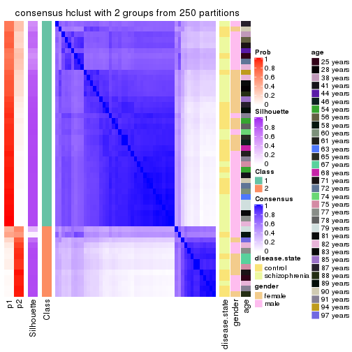
consensus_heatmap(res, k = 3)
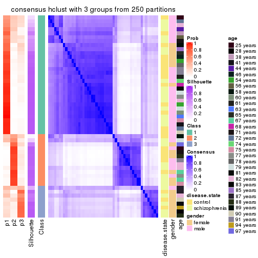
consensus_heatmap(res, k = 4)

consensus_heatmap(res, k = 5)
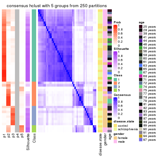
consensus_heatmap(res, k = 6)
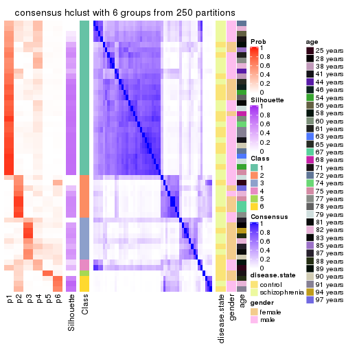
Heatmaps for the membership of samples in all partitions to see how consistent they are:
membership_heatmap(res, k = 2)
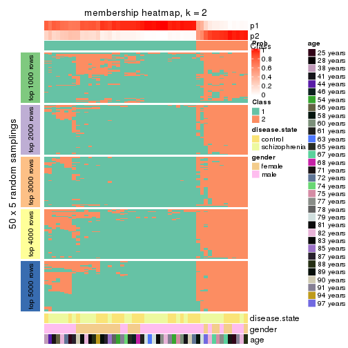
membership_heatmap(res, k = 3)
membership_heatmap(res, k = 4)
membership_heatmap(res, k = 5)
membership_heatmap(res, k = 6)
As soon as we have had the classes for columns, we can look for signatures which are significantly different between classes which can be candidate marks for certain classes. Following are the heatmaps for signatures.
Signature heatmaps where rows are scaled:
get_signatures(res, k = 2)
get_signatures(res, k = 3)
get_signatures(res, k = 4)
get_signatures(res, k = 5)
get_signatures(res, k = 6)
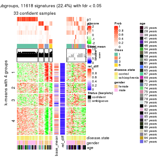
Signature heatmaps where rows are not scaled:
get_signatures(res, k = 2, scale_rows = FALSE)
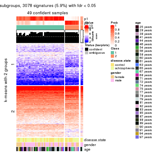
get_signatures(res, k = 3, scale_rows = FALSE)
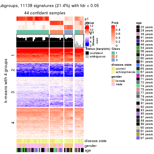
get_signatures(res, k = 4, scale_rows = FALSE)
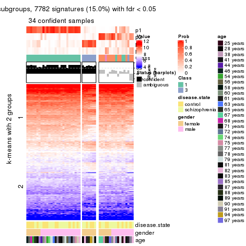
get_signatures(res, k = 5, scale_rows = FALSE)
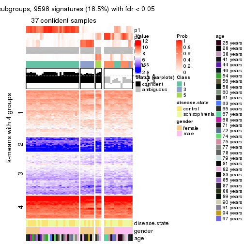
get_signatures(res, k = 6, scale_rows = FALSE)
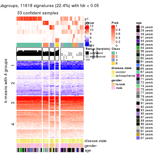
Compare the overlap of signatures from different k:
compare_signatures(res)
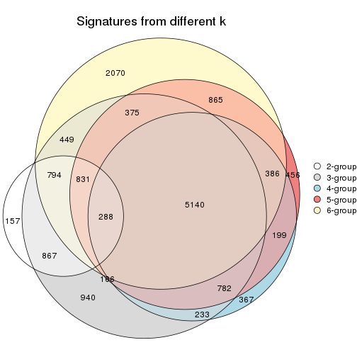
get_signature() returns a data frame invisibly. TO get the list of signatures, the function
call should be assigned to a variable explicitly. In following code, if plot argument is set
to FALSE, no heatmap is plotted while only the differential analysis is performed.
# code only for demonstration
tb = get_signature(res, k = ..., plot = FALSE)
An example of the output of tb is:
#>   which_row         fdr    mean_1    mean_2 scaled_mean_1 scaled_mean_2 km
#> 1        38 0.042760348  8.373488  9.131774    -0.5533452     0.5164555  1
#> 2        40 0.018707592  7.106213  8.469186    -0.6173731     0.5762149  1
#> 3        55 0.019134737 10.221463 11.207825    -0.6159697     0.5749050  1
#> 4        59 0.006059896  5.921854  7.869574    -0.6899429     0.6439467  1
#> 5        60 0.018055526  8.928898 10.211722    -0.6204761     0.5791110  1
#> 6        98 0.009384629 15.714769 14.887706     0.6635654    -0.6193277  2
...
The columns in tb are:
which_row: row indices corresponding to the input matrix.fdr: FDR for the differential test. mean_x: The mean value in group x.scaled_mean_x: The mean value in group x after rows are scaled.km: Row groups if k-means clustering is applied to rows.UMAP plot which shows how samples are separated.
dimension_reduction(res, k = 2, method = "UMAP")
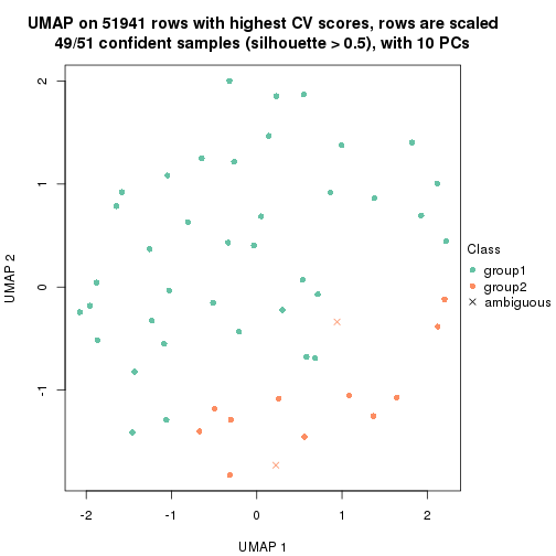
dimension_reduction(res, k = 3, method = "UMAP")
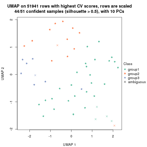
dimension_reduction(res, k = 4, method = "UMAP")
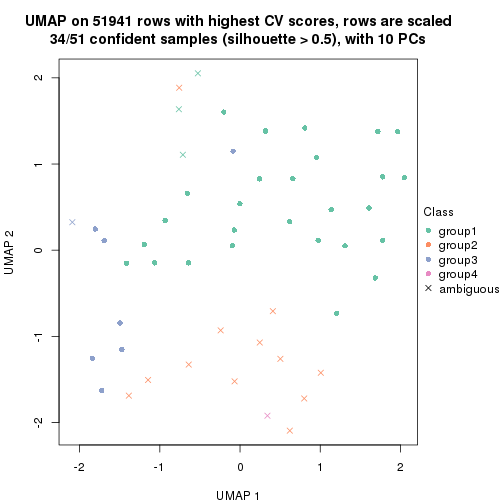
dimension_reduction(res, k = 5, method = "UMAP")
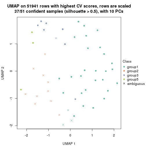
dimension_reduction(res, k = 6, method = "UMAP")
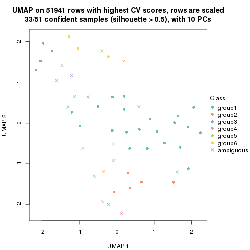
Following heatmap shows how subgroups are split when increasing k:
collect_classes(res)
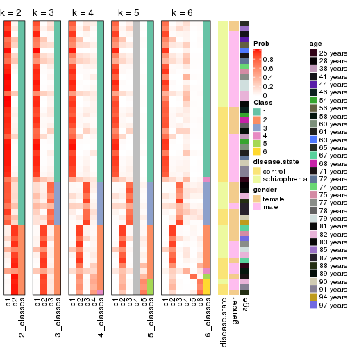
Test correlation between subgroups and known annotations. If the known annotation is numeric, one-way ANOVA test is applied, and if the known annotation is discrete, chi-squared contingency table test is applied.
test_to_known_factors(res)
#>            n disease.state(p) gender(p) age(p) k
#> CV:hclust 49            1.000   0.48161  0.814 2
#> CV:hclust 44            0.931   0.00206  0.603 3
#> CV:hclust 34            1.000   0.00182  0.471 4
#> CV:hclust 37            0.784   0.00173  0.947 5
#> CV:hclust 33            0.469   0.05006  0.674 6
If matrix rows can be associated to genes, consider to use functional_enrichment(res,
...) to perform function enrichment for the signature genes. See this vignette for more detailed explanations.
The object with results only for a single top-value method and a single partition method can be extracted as:
res = res_list["CV", "kmeans"]
# you can also extract it by
# res = res_list["CV:kmeans"]
A summary of res and all the functions that can be applied to it:
res
#> A 'ConsensusPartition' object with k = 2, 3, 4, 5, 6.
#>   On a matrix with 51941 rows and 51 columns.
#>   Top rows (1000, 2000, 3000, 4000, 5000) are extracted by 'CV' method.
#>   Subgroups are detected by 'kmeans' method.
#>   Performed in total 1250 partitions by row resampling.
#>   Best k for subgroups seems to be 2.
#>
#> Following methods can be applied to this 'ConsensusPartition' object:
#>  [1] "cola_report"             "collect_classes"         "collect_plots"
#>  [4] "collect_stats"           "colnames"                "compare_signatures"
#>  [7] "consensus_heatmap"       "dimension_reduction"     "functional_enrichment"
#> [10] "get_anno_col"            "get_anno"                "get_classes"
#> [13] "get_consensus"           "get_matrix"              "get_membership"
#> [16] "get_param"               "get_signatures"          "get_stats"
#> [19] "is_best_k"               "is_stable_k"             "membership_heatmap"
#> [22] "ncol"                    "nrow"                    "plot_ecdf"
#> [25] "rownames"                "select_partition_number" "show"
#> [28] "suggest_best_k"          "test_to_known_factors"
collect_plots() function collects all the plots made from res for all k (number of partitions)
into one single page to provide an easy and fast comparison between different k.
collect_plots(res)
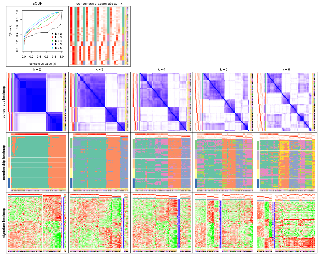
The plots are:
k and the heatmap of
predicted classes for each k.k.k.k.All the plots in panels can be made by individual functions and they are plotted later in this section.
select_partition_number() produces several plots showing different
statistics for choosing “optimized” k. There are following statistics:
k;k, the area increased is defined as \(A_k - A_{k-1}\).The detailed explanations of these statistics can be found in the cola vignette.
Generally speaking, lower PAC score, higher mean silhouette score or higher
concordance corresponds to better partition. Rand index and Jaccard index
measure how similar the current partition is compared to partition with k-1.
If they are too similar, we won't accept k is better than k-1.
select_partition_number(res)
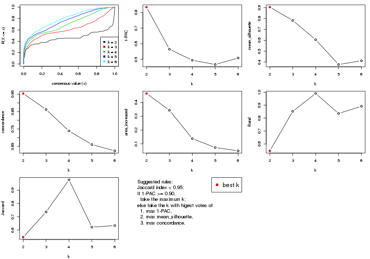
The numeric values for all these statistics can be obtained by get_stats().
get_stats(res)
#>   k 1-PAC mean_silhouette concordance area_increased  Rand Jaccard
#> 2 2 0.834           0.904       0.954         0.4642 0.547   0.547
#> 3 3 0.565           0.782       0.862         0.3429 0.853   0.736
#> 4 4 0.495           0.605       0.738         0.1376 0.991   0.978
#> 5 5 0.467           0.377       0.660         0.0733 0.836   0.622
#> 6 6 0.509           0.412       0.624         0.0494 0.892   0.634
suggest_best_k() suggests the best \(k\) based on these statistics. The rules are as follows:
suggest_best_k(res)
#> [1] 2
Following shows the table of the partitions (You need to click the show/hide
code output link to see it). The membership matrix (columns with name p*)
is inferred by
clue::cl_consensus()
function with the SE method. Basically the value in the membership matrix
represents the probability to belong to a certain group. The finall class
label for an item is determined with the group with highest probability it
belongs to.
In get_classes() function, the entropy is calculated from the membership
matrix and the silhouette score is calculated from the consensus matrix.
cbind(get_classes(res, k = 2), get_membership(res, k = 2))
#>           class entropy silhouette    p1    p2
#> GSM439800     1  0.8499      0.652 0.724 0.276
#> GSM439790     1  0.1414      0.940 0.980 0.020
#> GSM439827     2  0.0000      0.956 0.000 1.000
#> GSM439811     2  0.0000      0.956 0.000 1.000
#> GSM439795     2  0.3584      0.911 0.068 0.932
#> GSM439805     1  0.9427      0.494 0.640 0.360
#> GSM439781     1  0.3584      0.907 0.932 0.068
#> GSM439807     1  0.9460      0.483 0.636 0.364
#> GSM439820     2  0.0000      0.956 0.000 1.000
#> GSM439784     1  0.0000      0.947 1.000 0.000
#> GSM439824     1  0.8608      0.594 0.716 0.284
#> GSM439794     1  0.3274      0.906 0.940 0.060
#> GSM439809     1  0.0000      0.947 1.000 0.000
#> GSM439785     1  0.0376      0.946 0.996 0.004
#> GSM439803     1  0.0376      0.946 0.996 0.004
#> GSM439778     1  0.0000      0.947 1.000 0.000
#> GSM439791     1  0.0000      0.947 1.000 0.000
#> GSM439786     1  0.0000      0.947 1.000 0.000
#> GSM439828     2  0.0938      0.955 0.012 0.988
#> GSM439806     1  0.0000      0.947 1.000 0.000
#> GSM439815     1  0.0000      0.947 1.000 0.000
#> GSM439817     2  0.6801      0.793 0.180 0.820
#> GSM439796     1  0.0672      0.944 0.992 0.008
#> GSM439798     1  0.0000      0.947 1.000 0.000
#> GSM439821     2  0.0938      0.955 0.012 0.988
#> GSM439823     2  0.1633      0.950 0.024 0.976
#> GSM439813     1  0.0000      0.947 1.000 0.000
#> GSM439801     2  0.8386      0.665 0.268 0.732
#> GSM439810     1  0.1414      0.940 0.980 0.020
#> GSM439783     1  0.1414      0.940 0.980 0.020
#> GSM439826     2  0.0000      0.956 0.000 1.000
#> GSM439812     1  0.1414      0.940 0.980 0.020
#> GSM439818     2  0.0000      0.956 0.000 1.000
#> GSM439792     1  0.1414      0.940 0.980 0.020
#> GSM439802     1  0.5294      0.856 0.880 0.120
#> GSM439825     2  0.0000      0.956 0.000 1.000
#> GSM439780     1  0.1414      0.940 0.980 0.020
#> GSM439787     2  0.3114      0.922 0.056 0.944
#> GSM439808     2  0.0000      0.956 0.000 1.000
#> GSM439804     1  0.0376      0.946 0.996 0.004
#> GSM439822     2  0.0938      0.955 0.012 0.988
#> GSM439816     1  0.0376      0.946 0.996 0.004
#> GSM439789     1  0.0000      0.947 1.000 0.000
#> GSM439799     2  0.2043      0.946 0.032 0.968
#> GSM439814     1  0.0000      0.947 1.000 0.000
#> GSM439782     1  0.0000      0.947 1.000 0.000
#> GSM439779     1  0.0000      0.947 1.000 0.000
#> GSM439793     1  0.0000      0.947 1.000 0.000
#> GSM439788     1  0.0000      0.947 1.000 0.000
#> GSM439797     1  0.0376      0.946 0.996 0.004
#> GSM439819     2  0.0938      0.955 0.012 0.988
cbind(get_classes(res, k = 3), get_membership(res, k = 3))
#>           class entropy silhouette    p1    p2    p3
#> GSM439800     3  0.3045      0.846 0.064 0.020 0.916
#> GSM439790     1  0.5621      0.657 0.692 0.000 0.308
#> GSM439827     2  0.1529      0.904 0.000 0.960 0.040
#> GSM439811     2  0.1643      0.903 0.000 0.956 0.044
#> GSM439795     3  0.3213      0.857 0.008 0.092 0.900
#> GSM439805     3  0.3764      0.868 0.040 0.068 0.892
#> GSM439781     1  0.7043      0.293 0.532 0.020 0.448
#> GSM439807     3  0.3832      0.867 0.036 0.076 0.888
#> GSM439820     2  0.2959      0.885 0.000 0.900 0.100
#> GSM439784     1  0.1525      0.839 0.964 0.004 0.032
#> GSM439824     1  0.6925      0.173 0.532 0.452 0.016
#> GSM439794     1  0.7159      0.605 0.660 0.052 0.288
#> GSM439809     1  0.0983      0.840 0.980 0.004 0.016
#> GSM439785     1  0.3856      0.825 0.888 0.040 0.072
#> GSM439803     1  0.5778      0.740 0.768 0.032 0.200
#> GSM439778     1  0.2261      0.840 0.932 0.000 0.068
#> GSM439791     1  0.1129      0.840 0.976 0.004 0.020
#> GSM439786     1  0.4931      0.750 0.784 0.004 0.212
#> GSM439828     2  0.0237      0.908 0.004 0.996 0.000
#> GSM439806     1  0.1129      0.839 0.976 0.004 0.020
#> GSM439815     1  0.2400      0.839 0.932 0.004 0.064
#> GSM439817     2  0.3769      0.797 0.104 0.880 0.016
#> GSM439796     1  0.6646      0.678 0.712 0.048 0.240
#> GSM439798     1  0.4883      0.752 0.788 0.004 0.208
#> GSM439821     2  0.2301      0.905 0.004 0.936 0.060
#> GSM439823     2  0.1267      0.902 0.004 0.972 0.024
#> GSM439813     1  0.1643      0.840 0.956 0.000 0.044
#> GSM439801     3  0.7777      0.631 0.160 0.164 0.676
#> GSM439810     1  0.4121      0.782 0.832 0.000 0.168
#> GSM439783     1  0.4682      0.770 0.804 0.004 0.192
#> GSM439826     2  0.0747      0.909 0.000 0.984 0.016
#> GSM439812     1  0.3851      0.797 0.860 0.004 0.136
#> GSM439818     2  0.2625      0.897 0.000 0.916 0.084
#> GSM439792     1  0.3784      0.792 0.864 0.004 0.132
#> GSM439802     3  0.2400      0.823 0.064 0.004 0.932
#> GSM439825     2  0.2261      0.903 0.000 0.932 0.068
#> GSM439780     1  0.6500      0.351 0.532 0.004 0.464
#> GSM439787     3  0.3965      0.835 0.008 0.132 0.860
#> GSM439808     3  0.4931      0.721 0.000 0.232 0.768
#> GSM439804     1  0.6255      0.724 0.748 0.048 0.204
#> GSM439822     2  0.0661      0.909 0.004 0.988 0.008
#> GSM439816     1  0.2703      0.823 0.928 0.056 0.016
#> GSM439789     1  0.0892      0.839 0.980 0.000 0.020
#> GSM439799     2  0.6673      0.464 0.020 0.636 0.344
#> GSM439814     1  0.1163      0.839 0.972 0.000 0.028
#> GSM439782     1  0.2878      0.836 0.904 0.000 0.096
#> GSM439779     1  0.1031      0.840 0.976 0.000 0.024
#> GSM439793     1  0.1878      0.839 0.952 0.004 0.044
#> GSM439788     1  0.1878      0.839 0.952 0.004 0.044
#> GSM439797     1  0.3572      0.826 0.900 0.040 0.060
#> GSM439819     2  0.2200      0.907 0.004 0.940 0.056
cbind(get_classes(res, k = 4), get_membership(res, k = 4))
#>           class entropy silhouette    p1    p2    p3    p4
#> GSM439800     3   0.437     0.7500 0.016 0.020 0.808 0.156
#> GSM439790     1   0.741     0.4823 0.504 0.000 0.200 0.296
#> GSM439827     2   0.301     0.7457 0.000 0.892 0.052 0.056
#> GSM439811     2   0.309     0.7422 0.000 0.888 0.056 0.056
#> GSM439795     3   0.183     0.7399 0.000 0.024 0.944 0.032
#> GSM439805     3   0.398     0.7629 0.032 0.016 0.848 0.104
#> GSM439781     1   0.807     0.3042 0.444 0.012 0.300 0.244
#> GSM439807     3   0.418     0.7642 0.024 0.016 0.828 0.132
#> GSM439820     2   0.416     0.7061 0.000 0.828 0.096 0.076
#> GSM439784     1   0.254     0.7120 0.904 0.000 0.012 0.084
#> GSM439824     1   0.751     0.0365 0.460 0.348 0.000 0.192
#> GSM439794     1   0.729     0.3500 0.460 0.008 0.116 0.416
#> GSM439809     1   0.281     0.6993 0.868 0.000 0.000 0.132
#> GSM439785     1   0.498     0.5927 0.652 0.004 0.004 0.340
#> GSM439803     1   0.641     0.4424 0.516 0.008 0.048 0.428
#> GSM439778     1   0.389     0.7043 0.796 0.000 0.008 0.196
#> GSM439791     1   0.130     0.7161 0.956 0.000 0.000 0.044
#> GSM439786     1   0.638     0.5542 0.536 0.004 0.056 0.404
#> GSM439828     2   0.102     0.7533 0.000 0.968 0.000 0.032
#> GSM439806     1   0.234     0.7074 0.900 0.000 0.000 0.100
#> GSM439815     1   0.423     0.6885 0.760 0.000 0.008 0.232
#> GSM439817     2   0.399     0.5848 0.048 0.832 0.000 0.120
#> GSM439796     1   0.679     0.4002 0.488 0.008 0.072 0.432
#> GSM439798     1   0.633     0.5689 0.556 0.004 0.056 0.384
#> GSM439821     2   0.517     0.6252 0.000 0.760 0.116 0.124
#> GSM439823     2   0.281     0.6426 0.000 0.868 0.000 0.132
#> GSM439813     1   0.397     0.6826 0.788 0.000 0.008 0.204
#> GSM439801     3   0.809     0.0939 0.084 0.104 0.552 0.260
#> GSM439810     1   0.581     0.6472 0.708 0.000 0.132 0.160
#> GSM439783     1   0.548     0.6682 0.736 0.000 0.144 0.120
#> GSM439826     2   0.228     0.7588 0.000 0.924 0.024 0.052
#> GSM439812     1   0.460     0.6697 0.776 0.000 0.040 0.184
#> GSM439818     2   0.590     0.5799 0.000 0.700 0.156 0.144
#> GSM439792     1   0.394     0.6953 0.840 0.000 0.100 0.060
#> GSM439802     3   0.429     0.7239 0.036 0.000 0.800 0.164
#> GSM439825     2   0.566     0.6029 0.000 0.720 0.124 0.156
#> GSM439780     1   0.781     0.3039 0.408 0.000 0.264 0.328
#> GSM439787     3   0.209     0.7485 0.012 0.024 0.940 0.024
#> GSM439808     3   0.441     0.6818 0.000 0.128 0.808 0.064
#> GSM439804     1   0.642     0.4360 0.512 0.008 0.048 0.432
#> GSM439822     2   0.166     0.7541 0.000 0.944 0.004 0.052
#> GSM439816     1   0.517     0.6077 0.724 0.048 0.000 0.228
#> GSM439789     1   0.234     0.7057 0.900 0.000 0.000 0.100
#> GSM439799     4   0.777     0.0000 0.000 0.372 0.240 0.388
#> GSM439814     1   0.283     0.6936 0.876 0.000 0.004 0.120
#> GSM439782     1   0.498     0.6301 0.612 0.000 0.004 0.384
#> GSM439779     1   0.158     0.7141 0.948 0.000 0.004 0.048
#> GSM439793     1   0.328     0.7075 0.860 0.000 0.016 0.124
#> GSM439788     1   0.360     0.7046 0.836 0.000 0.016 0.148
#> GSM439797     1   0.540     0.5680 0.600 0.012 0.004 0.384
#> GSM439819     2   0.381     0.7098 0.000 0.848 0.060 0.092
cbind(get_classes(res, k = 5), get_membership(res, k = 5))
#>           class entropy silhouette    p1    p2    p3    p4    p5
#> GSM439800     3  0.4765    0.77735 0.008 0.004 0.756 0.140 0.092
#> GSM439790     1  0.8106    0.27526 0.380 0.000 0.240 0.272 0.108
#> GSM439827     2  0.3053    0.36244 0.000 0.872 0.044 0.008 0.076
#> GSM439811     2  0.2992    0.36553 0.000 0.876 0.044 0.008 0.072
#> GSM439795     3  0.3605    0.81752 0.000 0.012 0.832 0.036 0.120
#> GSM439805     3  0.4307    0.79663 0.012 0.008 0.804 0.100 0.076
#> GSM439781     1  0.8628    0.20199 0.324 0.012 0.304 0.220 0.140
#> GSM439807     3  0.2769    0.82797 0.004 0.008 0.892 0.028 0.068
#> GSM439820     2  0.5191    0.14421 0.000 0.740 0.096 0.040 0.124
#> GSM439784     1  0.4700    0.52096 0.772 0.008 0.024 0.148 0.048
#> GSM439824     2  0.7233    0.00772 0.380 0.420 0.000 0.152 0.048
#> GSM439794     4  0.5281    0.59157 0.264 0.012 0.052 0.668 0.004
#> GSM439809     1  0.2291    0.57384 0.908 0.000 0.000 0.036 0.056
#> GSM439785     4  0.5315    0.28817 0.432 0.024 0.000 0.528 0.016
#> GSM439803     4  0.4726    0.60298 0.256 0.012 0.024 0.704 0.004
#> GSM439778     1  0.5144    0.45039 0.680 0.000 0.008 0.244 0.068
#> GSM439791     1  0.3310    0.55675 0.836 0.004 0.000 0.136 0.024
#> GSM439786     1  0.7986    0.19822 0.360 0.000 0.088 0.320 0.232
#> GSM439828     2  0.0693    0.38716 0.000 0.980 0.000 0.012 0.008
#> GSM439806     1  0.1997    0.58085 0.924 0.000 0.000 0.036 0.040
#> GSM439815     1  0.4664    0.49909 0.748 0.000 0.004 0.152 0.096
#> GSM439817     2  0.4346    0.35979 0.044 0.808 0.004 0.100 0.044
#> GSM439796     4  0.4547    0.60210 0.252 0.012 0.024 0.712 0.000
#> GSM439798     1  0.8135    0.20245 0.368 0.004 0.092 0.308 0.228
#> GSM439821     2  0.5390   -0.66425 0.000 0.524 0.016 0.028 0.432
#> GSM439823     2  0.3771    0.33464 0.000 0.796 0.000 0.164 0.040
#> GSM439813     1  0.4279    0.53460 0.784 0.000 0.004 0.108 0.104
#> GSM439801     4  0.7587   -0.21915 0.028 0.064 0.408 0.412 0.088
#> GSM439810     1  0.5384    0.53130 0.732 0.000 0.116 0.060 0.092
#> GSM439783     1  0.6402    0.46381 0.628 0.004 0.120 0.204 0.044
#> GSM439826     2  0.3002    0.37297 0.000 0.872 0.004 0.048 0.076
#> GSM439812     1  0.4506    0.53652 0.792 0.000 0.036 0.076 0.096
#> GSM439818     2  0.6277   -0.56708 0.000 0.520 0.068 0.036 0.376
#> GSM439792     1  0.4375    0.57070 0.796 0.000 0.084 0.096 0.024
#> GSM439802     3  0.3620    0.79114 0.000 0.000 0.824 0.068 0.108
#> GSM439825     5  0.4886    0.00000 0.000 0.468 0.016 0.004 0.512
#> GSM439780     1  0.8511    0.21216 0.296 0.000 0.292 0.220 0.192
#> GSM439787     3  0.3946    0.80082 0.000 0.032 0.816 0.028 0.124
#> GSM439808     3  0.3977    0.79604 0.000 0.060 0.820 0.020 0.100
#> GSM439804     4  0.4674    0.60257 0.248 0.012 0.024 0.712 0.004
#> GSM439822     2  0.3527    0.12258 0.000 0.792 0.000 0.016 0.192
#> GSM439816     1  0.6249    0.30272 0.648 0.100 0.000 0.184 0.068
#> GSM439789     1  0.3875    0.54304 0.792 0.000 0.000 0.160 0.048
#> GSM439799     4  0.7706    0.03669 0.000 0.176 0.132 0.496 0.196
#> GSM439814     1  0.3362    0.54150 0.844 0.000 0.000 0.076 0.080
#> GSM439782     1  0.7097    0.22709 0.428 0.000 0.040 0.384 0.148
#> GSM439779     1  0.3110    0.56523 0.856 0.000 0.004 0.112 0.028
#> GSM439793     1  0.5644    0.46435 0.684 0.008 0.032 0.216 0.060
#> GSM439788     1  0.5496    0.46857 0.684 0.000 0.028 0.212 0.076
#> GSM439797     4  0.6161    0.17094 0.408 0.024 0.004 0.504 0.060
#> GSM439819     2  0.4880   -0.28694 0.000 0.664 0.012 0.028 0.296
cbind(get_classes(res, k = 6), get_membership(res, k = 6))
#>           class entropy silhouette    p1    p2    p3    p4    p5    p6
#> GSM439800     3   0.581     0.6979 0.012 0.000 0.660 0.104 0.148 0.076
#> GSM439790     5   0.788     0.4622 0.288 0.000 0.144 0.176 0.364 0.028
#> GSM439827     2   0.215     0.4389 0.000 0.916 0.036 0.004 0.012 0.032
#> GSM439811     2   0.215     0.4389 0.000 0.916 0.036 0.004 0.012 0.032
#> GSM439795     3   0.238     0.7455 0.000 0.016 0.908 0.020 0.016 0.040
#> GSM439805     3   0.411     0.7071 0.016 0.004 0.812 0.068 0.064 0.036
#> GSM439781     5   0.839     0.3938 0.228 0.012 0.172 0.188 0.360 0.040
#> GSM439807     3   0.448     0.7322 0.004 0.028 0.768 0.008 0.128 0.064
#> GSM439820     2   0.541     0.2296 0.000 0.692 0.080 0.020 0.044 0.164
#> GSM439784     1   0.579     0.3873 0.568 0.000 0.000 0.184 0.232 0.016
#> GSM439824     2   0.744     0.1075 0.300 0.416 0.000 0.184 0.036 0.064
#> GSM439794     4   0.282     0.6556 0.096 0.000 0.016 0.868 0.008 0.012
#> GSM439809     1   0.241     0.4868 0.900 0.000 0.000 0.028 0.044 0.028
#> GSM439785     4   0.525     0.2283 0.300 0.000 0.000 0.592 0.100 0.008
#> GSM439803     4   0.216     0.6607 0.096 0.004 0.008 0.892 0.000 0.000
#> GSM439778     1   0.582     0.2292 0.520 0.000 0.008 0.300 0.172 0.000
#> GSM439791     1   0.516     0.4419 0.636 0.000 0.000 0.200 0.160 0.004
#> GSM439786     5   0.601     0.5621 0.176 0.000 0.016 0.172 0.608 0.028
#> GSM439828     2   0.276     0.3966 0.000 0.848 0.004 0.004 0.008 0.136
#> GSM439806     1   0.331     0.4866 0.820 0.000 0.000 0.048 0.128 0.004
#> GSM439815     1   0.449     0.3899 0.752 0.000 0.004 0.152 0.040 0.052
#> GSM439817     2   0.566     0.3561 0.044 0.696 0.000 0.068 0.068 0.124
#> GSM439796     4   0.215     0.6653 0.084 0.004 0.008 0.900 0.000 0.004
#> GSM439798     5   0.585     0.5466 0.188 0.000 0.012 0.160 0.616 0.024
#> GSM439821     6   0.430     0.5866 0.000 0.276 0.024 0.016 0.000 0.684
#> GSM439823     2   0.557     0.2010 0.000 0.620 0.000 0.136 0.028 0.216
#> GSM439813     1   0.409     0.4113 0.800 0.000 0.004 0.076 0.068 0.052
#> GSM439801     3   0.664     0.2003 0.016 0.016 0.424 0.408 0.020 0.116
#> GSM439810     1   0.549     0.2998 0.708 0.000 0.092 0.040 0.112 0.048
#> GSM439783     1   0.784     0.1602 0.428 0.004 0.100 0.268 0.148 0.052
#> GSM439826     2   0.289     0.4072 0.000 0.868 0.008 0.012 0.024 0.088
#> GSM439812     1   0.386     0.4352 0.828 0.004 0.012 0.044 0.060 0.052
#> GSM439818     2   0.724    -0.2799 0.000 0.452 0.068 0.040 0.128 0.312
#> GSM439792     1   0.668     0.3904 0.564 0.000 0.064 0.168 0.180 0.024
#> GSM439802     3   0.344     0.7110 0.000 0.000 0.820 0.040 0.124 0.016
#> GSM439825     6   0.587     0.4104 0.000 0.324 0.020 0.016 0.088 0.552
#> GSM439780     5   0.715     0.5424 0.196 0.000 0.172 0.084 0.516 0.032
#> GSM439787     3   0.289     0.7314 0.000 0.044 0.872 0.008 0.008 0.068
#> GSM439808     3   0.534     0.6999 0.000 0.088 0.708 0.012 0.116 0.076
#> GSM439804     4   0.221     0.6631 0.080 0.004 0.008 0.900 0.000 0.008
#> GSM439822     2   0.419    -0.2445 0.000 0.572 0.000 0.016 0.000 0.412
#> GSM439816     1   0.655     0.2901 0.536 0.144 0.000 0.260 0.024 0.036
#> GSM439789     1   0.427     0.5011 0.704 0.000 0.000 0.248 0.036 0.012
#> GSM439799     4   0.656     0.0478 0.000 0.048 0.088 0.544 0.040 0.280
#> GSM439814     1   0.301     0.4783 0.856 0.000 0.000 0.084 0.012 0.048
#> GSM439782     5   0.647     0.4342 0.288 0.000 0.004 0.292 0.404 0.012
#> GSM439779     1   0.512     0.4590 0.652 0.000 0.000 0.188 0.152 0.008
#> GSM439793     1   0.610     0.2709 0.492 0.000 0.000 0.232 0.264 0.012
#> GSM439788     1   0.614     0.1885 0.472 0.000 0.000 0.216 0.300 0.012
#> GSM439797     4   0.595     0.1382 0.244 0.004 0.000 0.536 0.208 0.008
#> GSM439819     6   0.415     0.4173 0.000 0.412 0.008 0.004 0.000 0.576
Heatmaps for the consensus matrix. It visualizes the probability of two samples to be in a same group.
consensus_heatmap(res, k = 2)
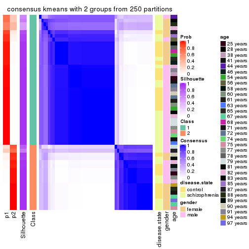
consensus_heatmap(res, k = 3)
consensus_heatmap(res, k = 4)
consensus_heatmap(res, k = 5)
consensus_heatmap(res, k = 6)
Heatmaps for the membership of samples in all partitions to see how consistent they are:
membership_heatmap(res, k = 2)
membership_heatmap(res, k = 3)
membership_heatmap(res, k = 4)
membership_heatmap(res, k = 5)
membership_heatmap(res, k = 6)
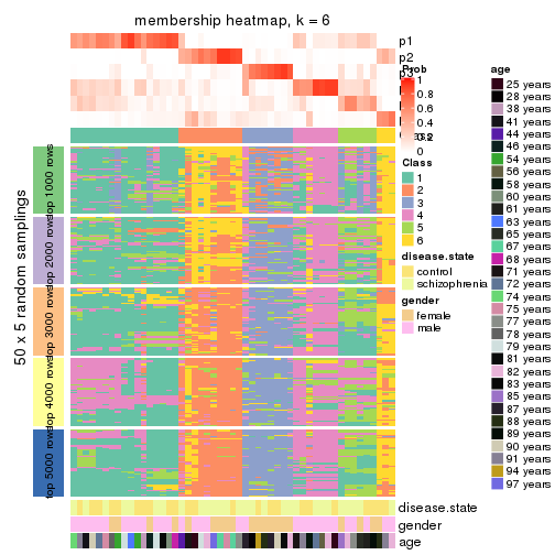
As soon as we have had the classes for columns, we can look for signatures which are significantly different between classes which can be candidate marks for certain classes. Following are the heatmaps for signatures.
Signature heatmaps where rows are scaled:
get_signatures(res, k = 2)
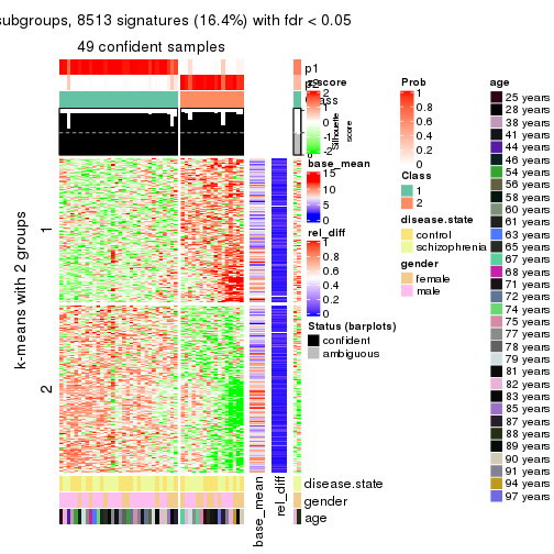
get_signatures(res, k = 3)
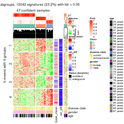
get_signatures(res, k = 4)
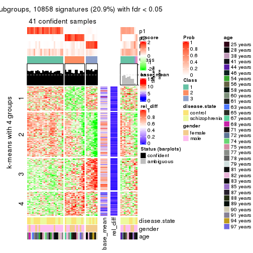
get_signatures(res, k = 5)
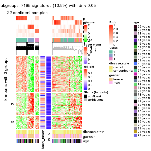
get_signatures(res, k = 6)
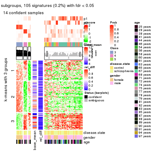
Signature heatmaps where rows are not scaled:
get_signatures(res, k = 2, scale_rows = FALSE)
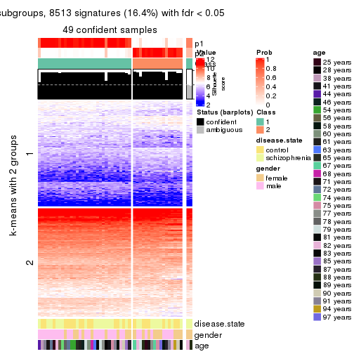
get_signatures(res, k = 3, scale_rows = FALSE)
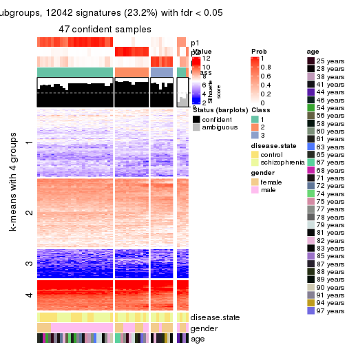
get_signatures(res, k = 4, scale_rows = FALSE)
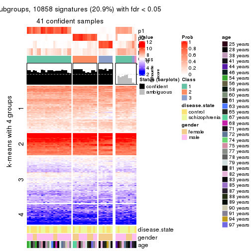
get_signatures(res, k = 5, scale_rows = FALSE)
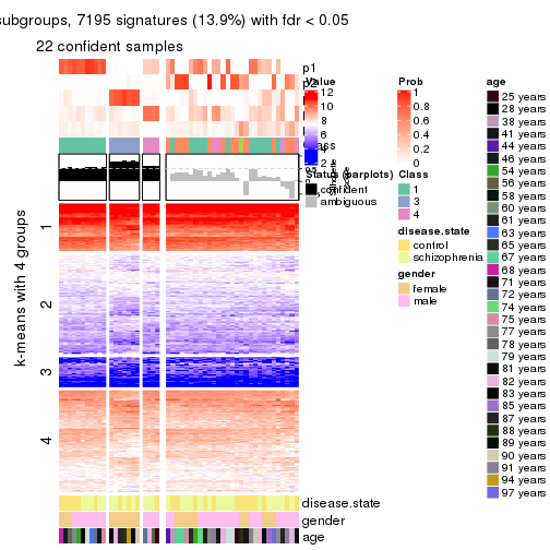
get_signatures(res, k = 6, scale_rows = FALSE)
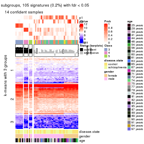
Compare the overlap of signatures from different k:
compare_signatures(res)
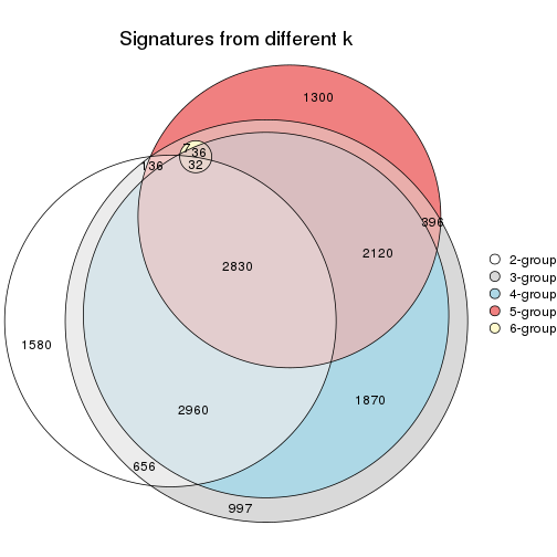
get_signature() returns a data frame invisibly. TO get the list of signatures, the function
call should be assigned to a variable explicitly. In following code, if plot argument is set
to FALSE, no heatmap is plotted while only the differential analysis is performed.
# code only for demonstration
tb = get_signature(res, k = ..., plot = FALSE)
An example of the output of tb is:
#>   which_row         fdr    mean_1    mean_2 scaled_mean_1 scaled_mean_2 km
#> 1        38 0.042760348  8.373488  9.131774    -0.5533452     0.5164555  1
#> 2        40 0.018707592  7.106213  8.469186    -0.6173731     0.5762149  1
#> 3        55 0.019134737 10.221463 11.207825    -0.6159697     0.5749050  1
#> 4        59 0.006059896  5.921854  7.869574    -0.6899429     0.6439467  1
#> 5        60 0.018055526  8.928898 10.211722    -0.6204761     0.5791110  1
#> 6        98 0.009384629 15.714769 14.887706     0.6635654    -0.6193277  2
...
The columns in tb are:
which_row: row indices corresponding to the input matrix.fdr: FDR for the differential test. mean_x: The mean value in group x.scaled_mean_x: The mean value in group x after rows are scaled.km: Row groups if k-means clustering is applied to rows.UMAP plot which shows how samples are separated.
dimension_reduction(res, k = 2, method = "UMAP")
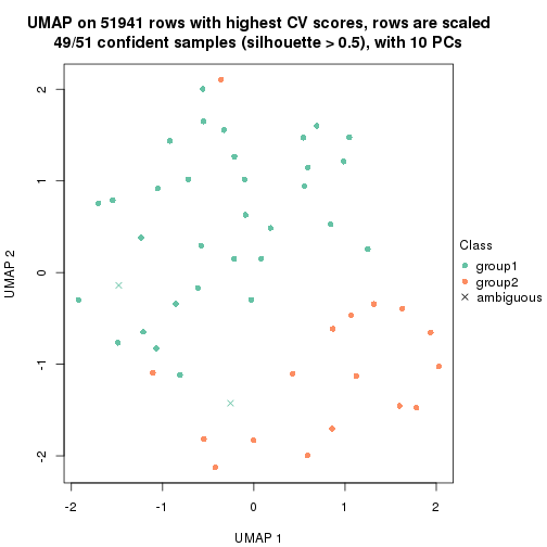
dimension_reduction(res, k = 3, method = "UMAP")
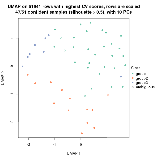
dimension_reduction(res, k = 4, method = "UMAP")
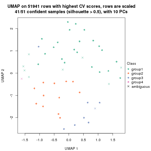
dimension_reduction(res, k = 5, method = "UMAP")
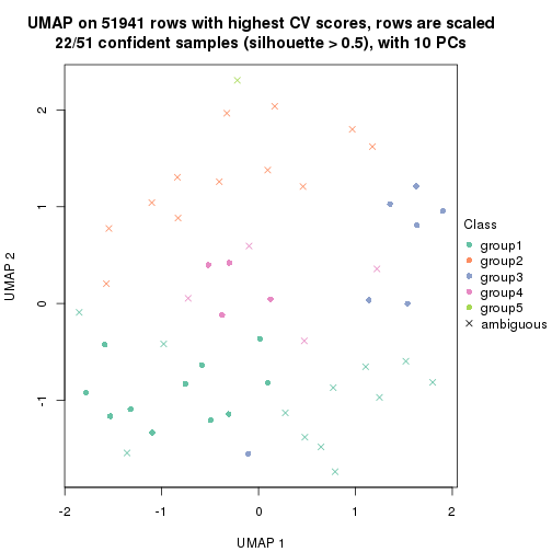
dimension_reduction(res, k = 6, method = "UMAP")
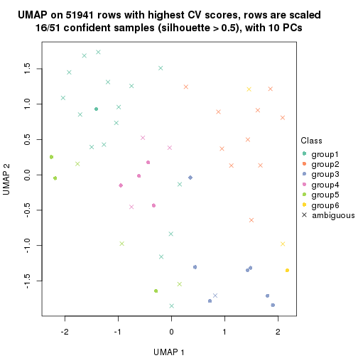
Following heatmap shows how subgroups are split when increasing k:
collect_classes(res)
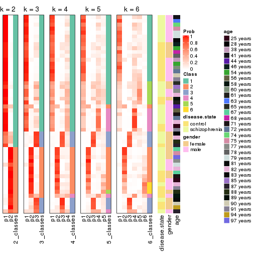
Test correlation between subgroups and known annotations. If the known annotation is numeric, one-way ANOVA test is applied, and if the known annotation is discrete, chi-squared contingency table test is applied.
test_to_known_factors(res)
#>            n disease.state(p) gender(p) age(p) k
#> CV:kmeans 49            1.000  0.160341  0.787 2
#> CV:kmeans 47            0.843  0.001255  0.515 3
#> CV:kmeans 41            0.728  0.000512  0.579 4
#> CV:kmeans 22            0.588  0.001360  0.566 5
#> CV:kmeans 16            0.620  0.009757  0.666 6
If matrix rows can be associated to genes, consider to use functional_enrichment(res,
...) to perform function enrichment for the signature genes. See this vignette for more detailed explanations.
The object with results only for a single top-value method and a single partition method can be extracted as:
res = res_list["CV", "skmeans"]
# you can also extract it by
# res = res_list["CV:skmeans"]
A summary of res and all the functions that can be applied to it:
res
#> A 'ConsensusPartition' object with k = 2, 3, 4, 5, 6.
#>   On a matrix with 51941 rows and 51 columns.
#>   Top rows (1000, 2000, 3000, 4000, 5000) are extracted by 'CV' method.
#>   Subgroups are detected by 'skmeans' method.
#>   Performed in total 1250 partitions by row resampling.
#>   Best k for subgroups seems to be 2.
#>
#> Following methods can be applied to this 'ConsensusPartition' object:
#>  [1] "cola_report"             "collect_classes"         "collect_plots"
#>  [4] "collect_stats"           "colnames"                "compare_signatures"
#>  [7] "consensus_heatmap"       "dimension_reduction"     "functional_enrichment"
#> [10] "get_anno_col"            "get_anno"                "get_classes"
#> [13] "get_consensus"           "get_matrix"              "get_membership"
#> [16] "get_param"               "get_signatures"          "get_stats"
#> [19] "is_best_k"               "is_stable_k"             "membership_heatmap"
#> [22] "ncol"                    "nrow"                    "plot_ecdf"
#> [25] "rownames"                "select_partition_number" "show"
#> [28] "suggest_best_k"          "test_to_known_factors"
collect_plots() function collects all the plots made from res for all k (number of partitions)
into one single page to provide an easy and fast comparison between different k.
collect_plots(res)
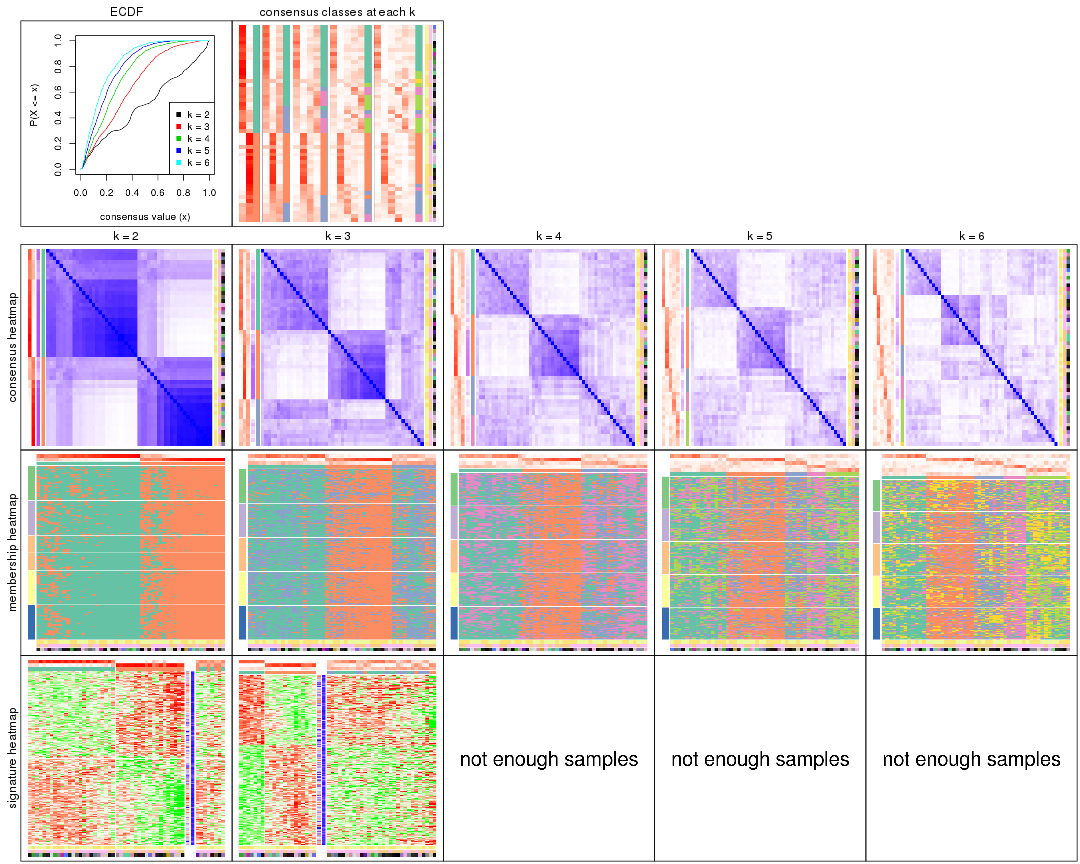
The plots are:
k and the heatmap of
predicted classes for each k.k.k.k.All the plots in panels can be made by individual functions and they are plotted later in this section.
select_partition_number() produces several plots showing different
statistics for choosing “optimized” k. There are following statistics:
k;k, the area increased is defined as \(A_k - A_{k-1}\).The detailed explanations of these statistics can be found in the cola vignette.
Generally speaking, lower PAC score, higher mean silhouette score or higher
concordance corresponds to better partition. Rand index and Jaccard index
measure how similar the current partition is compared to partition with k-1.
If they are too similar, we won't accept k is better than k-1.
select_partition_number(res)
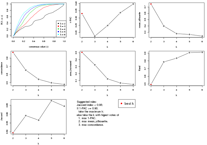
The numeric values for all these statistics can be obtained by get_stats().
get_stats(res)
#>   k 1-PAC mean_silhouette concordance area_increased  Rand Jaccard
#> 2 2 0.331           0.748       0.870         0.5058 0.495   0.495
#> 3 3 0.176           0.398       0.653         0.3266 0.787   0.592
#> 4 4 0.248           0.278       0.542         0.1236 0.835   0.566
#> 5 5 0.337           0.265       0.499         0.0649 0.907   0.676
#> 6 6 0.396           0.239       0.479         0.0438 0.911   0.645
suggest_best_k() suggests the best \(k\) based on these statistics. The rules are as follows:
suggest_best_k(res)
#> [1] 2
Following shows the table of the partitions (You need to click the show/hide
code output link to see it). The membership matrix (columns with name p*)
is inferred by
clue::cl_consensus()
function with the SE method. Basically the value in the membership matrix
represents the probability to belong to a certain group. The finall class
label for an item is determined with the group with highest probability it
belongs to.
In get_classes() function, the entropy is calculated from the membership
matrix and the silhouette score is calculated from the consensus matrix.
cbind(get_classes(res, k = 2), get_membership(res, k = 2))
#>           class entropy silhouette    p1    p2
#> GSM439800     2  0.9580      0.390 0.380 0.620
#> GSM439790     1  0.5408      0.834 0.876 0.124
#> GSM439827     2  0.0938      0.852 0.012 0.988
#> GSM439811     2  0.0938      0.852 0.012 0.988
#> GSM439795     2  0.3431      0.836 0.064 0.936
#> GSM439805     2  0.9044      0.536 0.320 0.680
#> GSM439781     1  0.9580      0.471 0.620 0.380
#> GSM439807     2  0.8955      0.539 0.312 0.688
#> GSM439820     2  0.0938      0.852 0.012 0.988
#> GSM439784     1  0.5946      0.813 0.856 0.144
#> GSM439824     2  0.9754      0.333 0.408 0.592
#> GSM439794     2  0.9608      0.423 0.384 0.616
#> GSM439809     1  0.1184      0.849 0.984 0.016
#> GSM439785     1  0.7139      0.761 0.804 0.196
#> GSM439803     1  0.7376      0.756 0.792 0.208
#> GSM439778     1  0.0000      0.843 1.000 0.000
#> GSM439791     1  0.1184      0.850 0.984 0.016
#> GSM439786     1  0.6048      0.818 0.852 0.148
#> GSM439828     2  0.0938      0.851 0.012 0.988
#> GSM439806     1  0.1843      0.853 0.972 0.028
#> GSM439815     1  0.3733      0.853 0.928 0.072
#> GSM439817     2  0.5842      0.791 0.140 0.860
#> GSM439796     2  0.9833      0.297 0.424 0.576
#> GSM439798     1  0.4690      0.845 0.900 0.100
#> GSM439821     2  0.0376      0.850 0.004 0.996
#> GSM439823     2  0.2948      0.843 0.052 0.948
#> GSM439813     1  0.1414      0.850 0.980 0.020
#> GSM439801     2  0.7219      0.736 0.200 0.800
#> GSM439810     1  0.4562      0.845 0.904 0.096
#> GSM439783     1  0.6343      0.808 0.840 0.160
#> GSM439826     2  0.1184      0.852 0.016 0.984
#> GSM439812     1  0.3584      0.853 0.932 0.068
#> GSM439818     2  0.0376      0.850 0.004 0.996
#> GSM439792     1  0.4562      0.846 0.904 0.096
#> GSM439802     1  0.9323      0.529 0.652 0.348
#> GSM439825     2  0.0000      0.849 0.000 1.000
#> GSM439780     1  0.2043      0.852 0.968 0.032
#> GSM439787     2  0.4161      0.825 0.084 0.916
#> GSM439808     2  0.1184      0.851 0.016 0.984
#> GSM439804     1  0.9661      0.403 0.608 0.392
#> GSM439822     2  0.0376      0.850 0.004 0.996
#> GSM439816     1  0.9427      0.489 0.640 0.360
#> GSM439789     1  0.0938      0.848 0.988 0.012
#> GSM439799     2  0.2043      0.848 0.032 0.968
#> GSM439814     1  0.1184      0.849 0.984 0.016
#> GSM439782     1  0.1414      0.851 0.980 0.020
#> GSM439779     1  0.0000      0.843 1.000 0.000
#> GSM439793     1  0.7674      0.738 0.776 0.224
#> GSM439788     1  0.3584      0.853 0.932 0.068
#> GSM439797     1  0.9661      0.394 0.608 0.392
#> GSM439819     2  0.0000      0.849 0.000 1.000
cbind(get_classes(res, k = 3), get_membership(res, k = 3))
#>           class entropy silhouette    p1    p2    p3
#> GSM439800     3   0.949     0.1929 0.184 0.400 0.416
#> GSM439790     3   0.775    -0.2030 0.452 0.048 0.500
#> GSM439827     2   0.503     0.7321 0.040 0.828 0.132
#> GSM439811     2   0.517     0.7042 0.016 0.792 0.192
#> GSM439795     2   0.815     0.2375 0.072 0.520 0.408
#> GSM439805     3   0.907     0.1788 0.140 0.384 0.476
#> GSM439781     3   0.947     0.1716 0.316 0.204 0.480
#> GSM439807     3   0.918     0.3449 0.168 0.324 0.508
#> GSM439820     2   0.422     0.7402 0.032 0.868 0.100
#> GSM439784     1   0.813     0.3265 0.600 0.096 0.304
#> GSM439824     2   0.927     0.0947 0.300 0.512 0.188
#> GSM439794     3   0.996     0.2832 0.292 0.340 0.368
#> GSM439809     1   0.582     0.5238 0.744 0.020 0.236
#> GSM439785     1   0.893     0.0917 0.452 0.124 0.424
#> GSM439803     1   0.867     0.1350 0.480 0.104 0.416
#> GSM439778     1   0.590     0.4877 0.680 0.004 0.316
#> GSM439791     1   0.639     0.4999 0.692 0.024 0.284
#> GSM439786     3   0.832    -0.1239 0.424 0.080 0.496
#> GSM439828     2   0.333     0.7516 0.020 0.904 0.076
#> GSM439806     1   0.486     0.5313 0.808 0.012 0.180
#> GSM439815     1   0.703     0.4272 0.676 0.052 0.272
#> GSM439817     2   0.677     0.6467 0.096 0.740 0.164
#> GSM439796     3   0.986     0.2546 0.296 0.288 0.416
#> GSM439798     3   0.788    -0.1955 0.424 0.056 0.520
#> GSM439821     2   0.196     0.7534 0.000 0.944 0.056
#> GSM439823     2   0.558     0.6968 0.040 0.792 0.168
#> GSM439813     1   0.549     0.5214 0.756 0.012 0.232
#> GSM439801     2   0.853     0.3056 0.116 0.564 0.320
#> GSM439810     1   0.646     0.4926 0.724 0.044 0.232
#> GSM439783     1   0.775     0.3731 0.596 0.064 0.340
#> GSM439826     2   0.308     0.7566 0.024 0.916 0.060
#> GSM439812     1   0.553     0.5044 0.792 0.036 0.172
#> GSM439818     2   0.268     0.7572 0.004 0.920 0.076
#> GSM439792     1   0.679     0.4422 0.648 0.028 0.324
#> GSM439802     3   0.861     0.1085 0.336 0.116 0.548
#> GSM439825     2   0.216     0.7547 0.000 0.936 0.064
#> GSM439780     1   0.729     0.2401 0.508 0.028 0.464
#> GSM439787     2   0.798     0.3731 0.076 0.584 0.340
#> GSM439808     2   0.671     0.5987 0.056 0.716 0.228
#> GSM439804     3   0.946     0.0114 0.396 0.180 0.424
#> GSM439822     2   0.212     0.7522 0.012 0.948 0.040
#> GSM439816     1   0.943    -0.1236 0.476 0.332 0.192
#> GSM439789     1   0.491     0.5288 0.804 0.012 0.184
#> GSM439799     2   0.586     0.6325 0.020 0.740 0.240
#> GSM439814     1   0.486     0.5368 0.820 0.020 0.160
#> GSM439782     1   0.665     0.4030 0.592 0.012 0.396
#> GSM439779     1   0.533     0.5306 0.748 0.004 0.248
#> GSM439793     1   0.856     0.2714 0.528 0.104 0.368
#> GSM439788     1   0.711     0.3811 0.584 0.028 0.388
#> GSM439797     3   0.956     0.1293 0.308 0.220 0.472
#> GSM439819     2   0.153     0.7526 0.004 0.964 0.032
cbind(get_classes(res, k = 4), get_membership(res, k = 4))
#>           class entropy silhouette    p1    p2    p3    p4
#> GSM439800     3   0.863     0.3044 0.188 0.216 0.512 0.084
#> GSM439790     1   0.838     0.0362 0.348 0.016 0.308 0.328
#> GSM439827     2   0.582     0.6106 0.028 0.748 0.120 0.104
#> GSM439811     2   0.625     0.5776 0.020 0.704 0.164 0.112
#> GSM439795     3   0.785     0.1980 0.060 0.292 0.548 0.100
#> GSM439805     3   0.871     0.2263 0.088 0.192 0.504 0.216
#> GSM439781     4   0.946     0.1387 0.212 0.132 0.256 0.400
#> GSM439807     3   0.938     0.1830 0.192 0.180 0.440 0.188
#> GSM439820     2   0.568     0.5936 0.036 0.720 0.216 0.028
#> GSM439784     4   0.796     0.0775 0.316 0.064 0.096 0.524
#> GSM439824     2   0.921     0.1058 0.196 0.444 0.120 0.240
#> GSM439794     3   0.978     0.1798 0.176 0.240 0.348 0.236
#> GSM439809     1   0.654     0.2245 0.616 0.028 0.048 0.308
#> GSM439785     4   0.905     0.1273 0.272 0.088 0.204 0.436
#> GSM439803     3   0.924     0.0377 0.296 0.100 0.400 0.204
#> GSM439778     1   0.696     0.1738 0.536 0.004 0.108 0.352
#> GSM439791     1   0.763     0.1063 0.444 0.020 0.120 0.416
#> GSM439786     4   0.867     0.1531 0.248 0.068 0.200 0.484
#> GSM439828     2   0.413     0.6532 0.028 0.852 0.068 0.052
#> GSM439806     1   0.692     0.2259 0.572 0.016 0.084 0.328
#> GSM439815     1   0.758     0.2701 0.584 0.028 0.188 0.200
#> GSM439817     2   0.742     0.5120 0.080 0.644 0.160 0.116
#> GSM439796     3   0.968     0.1426 0.204 0.192 0.384 0.220
#> GSM439798     4   0.759     0.2127 0.216 0.028 0.176 0.580
#> GSM439821     2   0.292     0.6537 0.000 0.884 0.100 0.016
#> GSM439823     2   0.590     0.5765 0.016 0.716 0.192 0.076
#> GSM439813     1   0.546     0.3369 0.752 0.008 0.096 0.144
#> GSM439801     3   0.874     0.0380 0.088 0.384 0.400 0.128
#> GSM439810     1   0.762     0.2766 0.560 0.020 0.192 0.228
#> GSM439783     1   0.874     0.0942 0.396 0.048 0.220 0.336
#> GSM439826     2   0.465     0.6474 0.028 0.820 0.104 0.048
#> GSM439812     1   0.713     0.3104 0.644 0.036 0.176 0.144
#> GSM439818     2   0.478     0.6158 0.000 0.752 0.212 0.036
#> GSM439792     1   0.839     0.1391 0.476 0.060 0.140 0.324
#> GSM439802     3   0.850    -0.0523 0.296 0.036 0.440 0.228
#> GSM439825     2   0.422     0.6422 0.008 0.808 0.164 0.020
#> GSM439780     1   0.814     0.0990 0.420 0.012 0.252 0.316
#> GSM439787     2   0.817     0.0942 0.032 0.440 0.368 0.160
#> GSM439808     2   0.748     0.2609 0.056 0.500 0.388 0.056
#> GSM439804     3   0.963     0.0955 0.304 0.152 0.348 0.196
#> GSM439822     2   0.312     0.6616 0.016 0.888 0.084 0.012
#> GSM439816     1   0.974    -0.0324 0.364 0.248 0.192 0.196
#> GSM439789     1   0.639     0.3150 0.692 0.020 0.116 0.172
#> GSM439799     2   0.748     0.3045 0.036 0.532 0.344 0.088
#> GSM439814     1   0.602     0.3163 0.708 0.024 0.064 0.204
#> GSM439782     1   0.741     0.2053 0.528 0.012 0.136 0.324
#> GSM439779     1   0.636     0.2017 0.544 0.004 0.056 0.396
#> GSM439793     4   0.714     0.2126 0.220 0.032 0.120 0.628
#> GSM439788     4   0.714     0.1783 0.232 0.028 0.120 0.620
#> GSM439797     4   0.868     0.2477 0.172 0.100 0.212 0.516
#> GSM439819     2   0.255     0.6589 0.000 0.900 0.092 0.008
cbind(get_classes(res, k = 5), get_membership(res, k = 5))
#>           class entropy silhouette    p1    p2    p3    p4    p5
#> GSM439800     3   0.897    0.22566 0.160 0.172 0.420 0.188 0.060
#> GSM439790     5   0.889    0.10354 0.224 0.016 0.272 0.188 0.300
#> GSM439827     2   0.699    0.51501 0.044 0.644 0.120 0.088 0.104
#> GSM439811     2   0.730    0.48167 0.044 0.612 0.152 0.096 0.096
#> GSM439795     3   0.702    0.29950 0.032 0.264 0.576 0.072 0.056
#> GSM439805     3   0.837    0.31245 0.072 0.124 0.512 0.176 0.116
#> GSM439781     5   0.910    0.15400 0.116 0.096 0.292 0.128 0.368
#> GSM439807     3   0.808    0.31153 0.120 0.116 0.556 0.092 0.116
#> GSM439820     2   0.736    0.40586 0.068 0.564 0.248 0.076 0.044
#> GSM439784     5   0.763   -0.01581 0.284 0.040 0.096 0.064 0.516
#> GSM439824     2   0.904    0.18463 0.180 0.416 0.068 0.172 0.164
#> GSM439794     4   0.928    0.24851 0.224 0.116 0.152 0.388 0.120
#> GSM439809     1   0.712    0.26069 0.576 0.028 0.052 0.100 0.244
#> GSM439785     4   0.800    0.15891 0.128 0.072 0.032 0.448 0.320
#> GSM439803     4   0.723    0.39559 0.108 0.064 0.076 0.628 0.124
#> GSM439778     1   0.835    0.07239 0.340 0.008 0.100 0.248 0.304
#> GSM439791     1   0.849    0.07880 0.344 0.016 0.108 0.212 0.320
#> GSM439786     5   0.834    0.20564 0.168 0.036 0.120 0.192 0.484
#> GSM439828     2   0.559    0.56474 0.008 0.732 0.104 0.088 0.068
#> GSM439806     1   0.760    0.21388 0.480 0.016 0.068 0.124 0.312
#> GSM439815     1   0.749    0.21760 0.532 0.024 0.080 0.268 0.096
#> GSM439817     2   0.789    0.40407 0.076 0.572 0.116 0.112 0.124
#> GSM439796     4   0.695    0.43320 0.116 0.116 0.060 0.648 0.060
#> GSM439798     5   0.725    0.27835 0.096 0.024 0.192 0.096 0.592
#> GSM439821     2   0.477    0.53597 0.004 0.768 0.136 0.068 0.024
#> GSM439823     2   0.641    0.51947 0.020 0.664 0.076 0.172 0.068
#> GSM439813     1   0.646    0.31539 0.636 0.000 0.076 0.160 0.128
#> GSM439801     2   0.865    0.00491 0.056 0.412 0.272 0.180 0.080
#> GSM439810     1   0.751    0.23578 0.560 0.016 0.184 0.104 0.136
#> GSM439783     1   0.880    0.07808 0.368 0.020 0.200 0.184 0.228
#> GSM439826     2   0.566    0.56448 0.028 0.724 0.092 0.132 0.024
#> GSM439812     1   0.543    0.35376 0.756 0.024 0.084 0.060 0.076
#> GSM439818     2   0.617    0.50061 0.020 0.664 0.196 0.088 0.032
#> GSM439792     1   0.813    0.16745 0.452 0.028 0.156 0.080 0.284
#> GSM439802     3   0.828   -0.02565 0.188 0.024 0.472 0.120 0.196
#> GSM439825     2   0.565    0.53464 0.024 0.716 0.148 0.092 0.020
#> GSM439780     5   0.890    0.09415 0.264 0.020 0.276 0.156 0.284
#> GSM439787     3   0.746    0.13396 0.012 0.340 0.464 0.056 0.128
#> GSM439808     2   0.752    0.15315 0.036 0.460 0.368 0.072 0.064
#> GSM439804     4   0.765    0.36943 0.224 0.084 0.052 0.556 0.084
#> GSM439822     2   0.393    0.58375 0.032 0.844 0.044 0.064 0.016
#> GSM439816     1   0.974   -0.04481 0.296 0.208 0.120 0.208 0.168
#> GSM439789     1   0.726    0.27309 0.564 0.016 0.076 0.232 0.112
#> GSM439799     2   0.769    0.26677 0.012 0.480 0.204 0.248 0.056
#> GSM439814     1   0.576    0.35050 0.720 0.012 0.060 0.088 0.120
#> GSM439782     1   0.876   -0.00774 0.324 0.016 0.144 0.256 0.260
#> GSM439779     1   0.758    0.18387 0.480 0.004 0.104 0.116 0.296
#> GSM439793     5   0.616    0.22497 0.140 0.020 0.060 0.088 0.692
#> GSM439788     5   0.769    0.15069 0.240 0.020 0.140 0.080 0.520
#> GSM439797     5   0.879   -0.07342 0.088 0.132 0.080 0.316 0.384
#> GSM439819     2   0.391    0.56977 0.000 0.828 0.096 0.044 0.032
cbind(get_classes(res, k = 6), get_membership(res, k = 6))
#>           class entropy silhouette    p1    p2    p3    p4    p5    p6
#> GSM439800     3   0.931   0.147849 0.144 0.168 0.348 0.164 0.076 0.100
#> GSM439790     5   0.867   0.144105 0.172 0.016 0.248 0.112 0.356 0.096
#> GSM439827     2   0.674   0.454858 0.032 0.560 0.096 0.024 0.032 0.256
#> GSM439811     2   0.721   0.400437 0.008 0.476 0.112 0.052 0.044 0.308
#> GSM439795     3   0.686   0.350521 0.036 0.228 0.580 0.068 0.040 0.048
#> GSM439805     3   0.837   0.277200 0.064 0.108 0.492 0.128 0.108 0.100
#> GSM439781     5   0.795   0.097518 0.048 0.048 0.288 0.048 0.436 0.132
#> GSM439807     3   0.739   0.274175 0.100 0.072 0.592 0.056 0.088 0.092
#> GSM439820     2   0.668   0.404705 0.024 0.588 0.152 0.044 0.016 0.176
#> GSM439784     5   0.821   0.002428 0.264 0.028 0.088 0.028 0.364 0.228
#> GSM439824     2   0.806  -0.034764 0.108 0.364 0.040 0.092 0.036 0.360
#> GSM439794     4   0.891   0.142547 0.152 0.092 0.148 0.420 0.084 0.104
#> GSM439809     1   0.704   0.296226 0.572 0.008 0.068 0.064 0.188 0.100
#> GSM439785     4   0.839   0.111871 0.092 0.040 0.052 0.424 0.212 0.180
#> GSM439803     4   0.640   0.329018 0.112 0.016 0.076 0.660 0.068 0.068
#> GSM439778     5   0.831  -0.050878 0.264 0.004 0.060 0.252 0.316 0.104
#> GSM439791     1   0.866   0.135247 0.332 0.028 0.044 0.152 0.260 0.184
#> GSM439786     5   0.806   0.220506 0.136 0.020 0.080 0.160 0.488 0.116
#> GSM439828     2   0.527   0.532343 0.004 0.692 0.032 0.048 0.024 0.200
#> GSM439806     1   0.790   0.220719 0.440 0.016 0.044 0.084 0.256 0.160
#> GSM439815     1   0.720   0.246411 0.556 0.012 0.052 0.196 0.104 0.080
#> GSM439817     2   0.846   0.278812 0.044 0.412 0.084 0.148 0.064 0.248
#> GSM439796     4   0.486   0.365779 0.080 0.024 0.040 0.776 0.028 0.052
#> GSM439798     5   0.639   0.269610 0.080 0.024 0.104 0.084 0.664 0.044
#> GSM439821     2   0.499   0.474566 0.008 0.744 0.128 0.060 0.016 0.044
#> GSM439823     2   0.719   0.380527 0.004 0.516 0.068 0.220 0.036 0.156
#> GSM439813     1   0.611   0.328987 0.656 0.004 0.032 0.112 0.136 0.060
#> GSM439801     3   0.873   0.165199 0.036 0.224 0.356 0.216 0.104 0.064
#> GSM439810     1   0.777   0.248627 0.488 0.004 0.080 0.092 0.180 0.156
#> GSM439783     1   0.938  -0.000937 0.256 0.028 0.188 0.176 0.172 0.180
#> GSM439826     2   0.660   0.496697 0.016 0.616 0.080 0.088 0.028 0.172
#> GSM439812     1   0.578   0.330238 0.712 0.020 0.088 0.044 0.056 0.080
#> GSM439818     2   0.576   0.438906 0.004 0.644 0.168 0.040 0.004 0.140
#> GSM439792     1   0.820   0.193662 0.424 0.024 0.112 0.040 0.180 0.220
#> GSM439802     3   0.776   0.068519 0.120 0.024 0.512 0.080 0.196 0.068
#> GSM439825     2   0.516   0.466836 0.012 0.724 0.124 0.044 0.004 0.092
#> GSM439780     5   0.844   0.114984 0.212 0.008 0.268 0.076 0.336 0.100
#> GSM439787     3   0.750   0.282635 0.024 0.224 0.488 0.012 0.100 0.152
#> GSM439808     3   0.769   0.047981 0.024 0.280 0.412 0.064 0.016 0.204
#> GSM439804     4   0.684   0.321177 0.116 0.040 0.052 0.632 0.084 0.076
#> GSM439822     2   0.379   0.555541 0.004 0.828 0.032 0.064 0.008 0.064
#> GSM439816     6   0.907   0.000000 0.248 0.192 0.044 0.132 0.076 0.308
#> GSM439789     1   0.705   0.250963 0.580 0.024 0.028 0.164 0.080 0.124
#> GSM439799     4   0.777  -0.033804 0.004 0.320 0.160 0.384 0.036 0.096
#> GSM439814     1   0.509   0.344984 0.756 0.016 0.024 0.064 0.084 0.056
#> GSM439782     5   0.817   0.003708 0.312 0.008 0.072 0.180 0.352 0.076
#> GSM439779     1   0.699   0.216331 0.456 0.000 0.028 0.080 0.340 0.096
#> GSM439793     5   0.785   0.181901 0.112 0.036 0.076 0.084 0.524 0.168
#> GSM439788     5   0.740   0.182517 0.136 0.004 0.092 0.092 0.548 0.128
#> GSM439797     5   0.824  -0.035105 0.040 0.092 0.016 0.240 0.344 0.268
#> GSM439819     2   0.433   0.531836 0.000 0.788 0.092 0.024 0.024 0.072
Heatmaps for the consensus matrix. It visualizes the probability of two samples to be in a same group.
consensus_heatmap(res, k = 2)
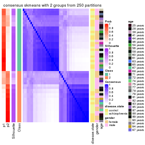
consensus_heatmap(res, k = 3)
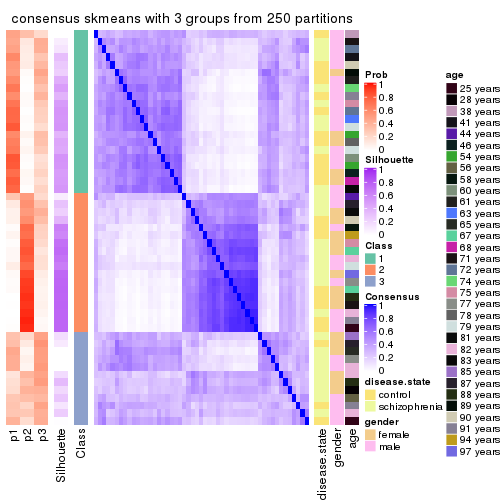
consensus_heatmap(res, k = 4)
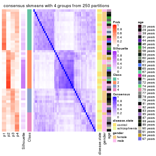
consensus_heatmap(res, k = 5)
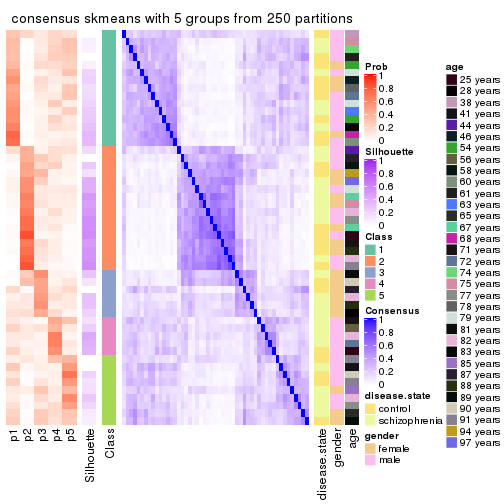
consensus_heatmap(res, k = 6)
Heatmaps for the membership of samples in all partitions to see how consistent they are:
membership_heatmap(res, k = 2)
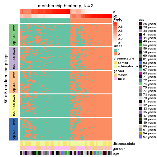
membership_heatmap(res, k = 3)
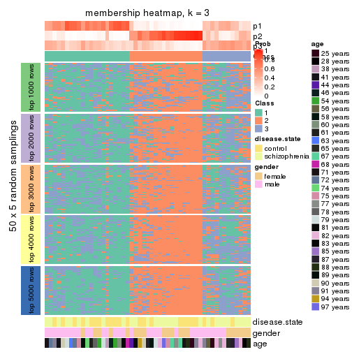
membership_heatmap(res, k = 4)
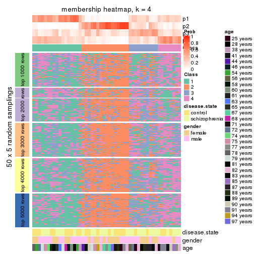
membership_heatmap(res, k = 5)
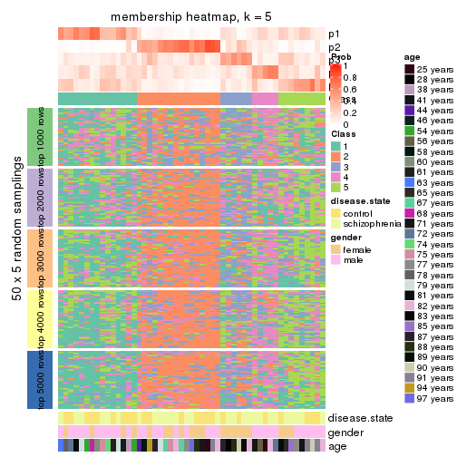
membership_heatmap(res, k = 6)
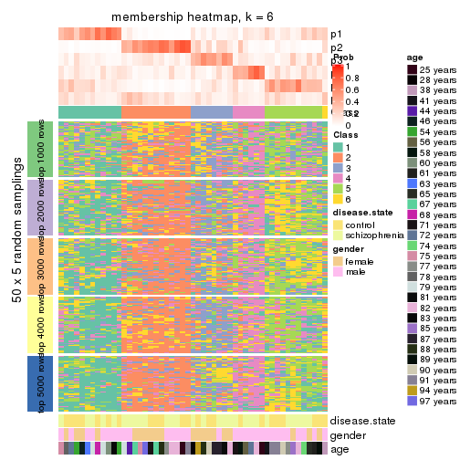
As soon as we have had the classes for columns, we can look for signatures which are significantly different between classes which can be candidate marks for certain classes. Following are the heatmaps for signatures.
Signature heatmaps where rows are scaled:
get_signatures(res, k = 2)
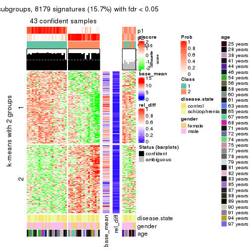
get_signatures(res, k = 3)
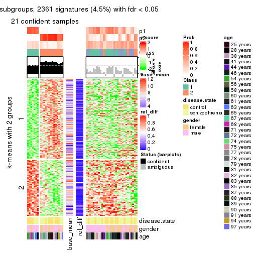
get_signatures(res, k = 4)

get_signatures(res, k = 5)

get_signatures(res, k = 6)

Signature heatmaps where rows are not scaled:
get_signatures(res, k = 2, scale_rows = FALSE)
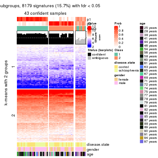
get_signatures(res, k = 3, scale_rows = FALSE)
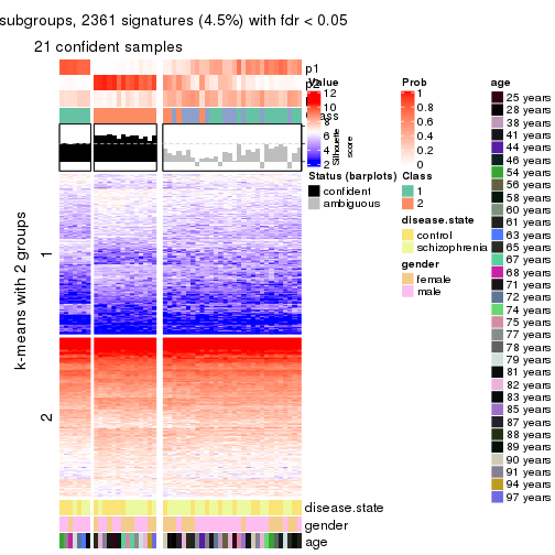
get_signatures(res, k = 4, scale_rows = FALSE)

get_signatures(res, k = 5, scale_rows = FALSE)

get_signatures(res, k = 6, scale_rows = FALSE)

Compare the overlap of signatures from different k:
compare_signatures(res)
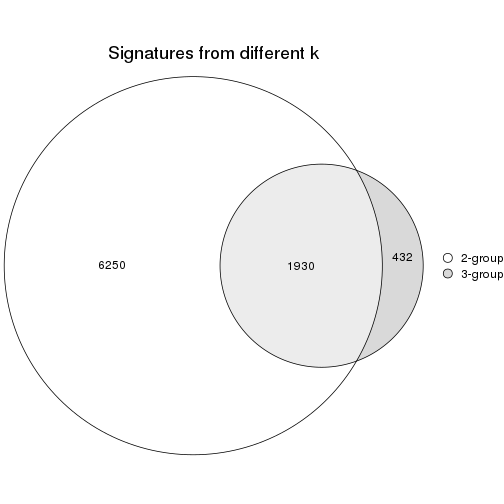
get_signature() returns a data frame invisibly. TO get the list of signatures, the function
call should be assigned to a variable explicitly. In following code, if plot argument is set
to FALSE, no heatmap is plotted while only the differential analysis is performed.
# code only for demonstration
tb = get_signature(res, k = ..., plot = FALSE)
An example of the output of tb is:
#>   which_row         fdr    mean_1    mean_2 scaled_mean_1 scaled_mean_2 km
#> 1        38 0.042760348  8.373488  9.131774    -0.5533452     0.5164555  1
#> 2        40 0.018707592  7.106213  8.469186    -0.6173731     0.5762149  1
#> 3        55 0.019134737 10.221463 11.207825    -0.6159697     0.5749050  1
#> 4        59 0.006059896  5.921854  7.869574    -0.6899429     0.6439467  1
#> 5        60 0.018055526  8.928898 10.211722    -0.6204761     0.5791110  1
#> 6        98 0.009384629 15.714769 14.887706     0.6635654    -0.6193277  2
...
The columns in tb are:
which_row: row indices corresponding to the input matrix.fdr: FDR for the differential test. mean_x: The mean value in group x.scaled_mean_x: The mean value in group x after rows are scaled.km: Row groups if k-means clustering is applied to rows.UMAP plot which shows how samples are separated.
dimension_reduction(res, k = 2, method = "UMAP")
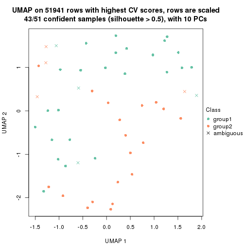
dimension_reduction(res, k = 3, method = "UMAP")
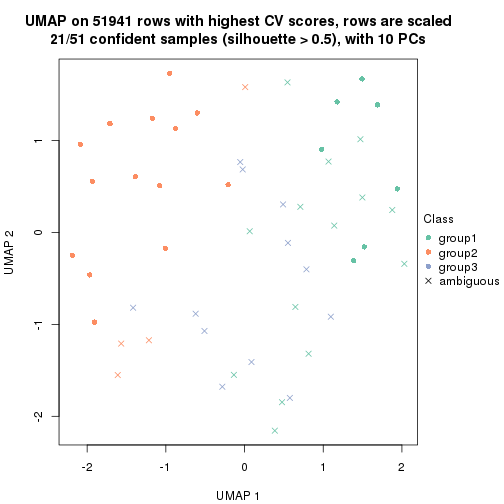
dimension_reduction(res, k = 4, method = "UMAP")
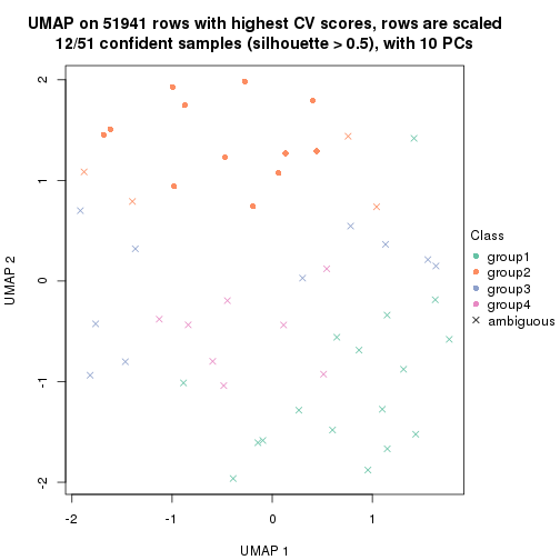
dimension_reduction(res, k = 5, method = "UMAP")
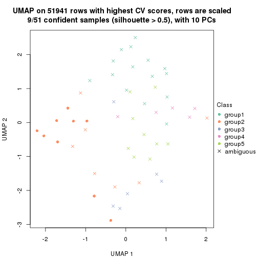
dimension_reduction(res, k = 6, method = "UMAP")
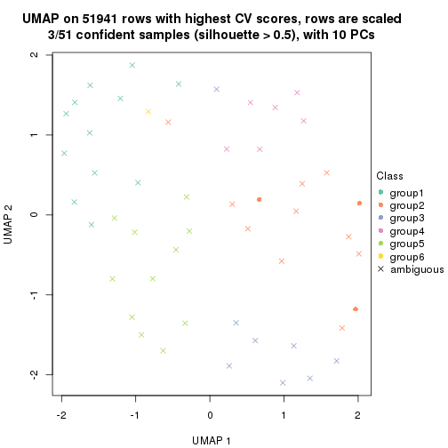
Following heatmap shows how subgroups are split when increasing k:
collect_classes(res)
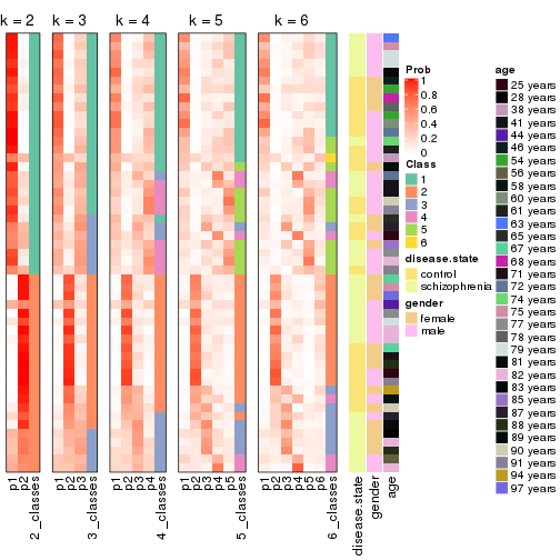
Test correlation between subgroups and known annotations. If the known annotation is numeric, one-way ANOVA test is applied, and if the known annotation is discrete, chi-squared contingency table test is applied.
test_to_known_factors(res)
#>             n disease.state(p) gender(p) age(p) k
#> CV:skmeans 43            0.836     0.113  0.569 2
#> CV:skmeans 21            1.000     0.266  0.343 3
#> CV:skmeans 12               NA        NA     NA 4
#> CV:skmeans  9               NA        NA     NA 5
#> CV:skmeans  3               NA        NA     NA 6
If matrix rows can be associated to genes, consider to use functional_enrichment(res,
...) to perform function enrichment for the signature genes. See this vignette for more detailed explanations.
The object with results only for a single top-value method and a single partition method can be extracted as:
res = res_list["CV", "pam"]
# you can also extract it by
# res = res_list["CV:pam"]
A summary of res and all the functions that can be applied to it:
res
#> A 'ConsensusPartition' object with k = 2, 3, 4, 5, 6.
#>   On a matrix with 51941 rows and 51 columns.
#>   Top rows (1000, 2000, 3000, 4000, 5000) are extracted by 'CV' method.
#>   Subgroups are detected by 'pam' method.
#>   Performed in total 1250 partitions by row resampling.
#>   Best k for subgroups seems to be 3.
#>
#> Following methods can be applied to this 'ConsensusPartition' object:
#>  [1] "cola_report"             "collect_classes"         "collect_plots"
#>  [4] "collect_stats"           "colnames"                "compare_signatures"
#>  [7] "consensus_heatmap"       "dimension_reduction"     "functional_enrichment"
#> [10] "get_anno_col"            "get_anno"                "get_classes"
#> [13] "get_consensus"           "get_matrix"              "get_membership"
#> [16] "get_param"               "get_signatures"          "get_stats"
#> [19] "is_best_k"               "is_stable_k"             "membership_heatmap"
#> [22] "ncol"                    "nrow"                    "plot_ecdf"
#> [25] "rownames"                "select_partition_number" "show"
#> [28] "suggest_best_k"          "test_to_known_factors"
collect_plots() function collects all the plots made from res for all k (number of partitions)
into one single page to provide an easy and fast comparison between different k.
collect_plots(res)
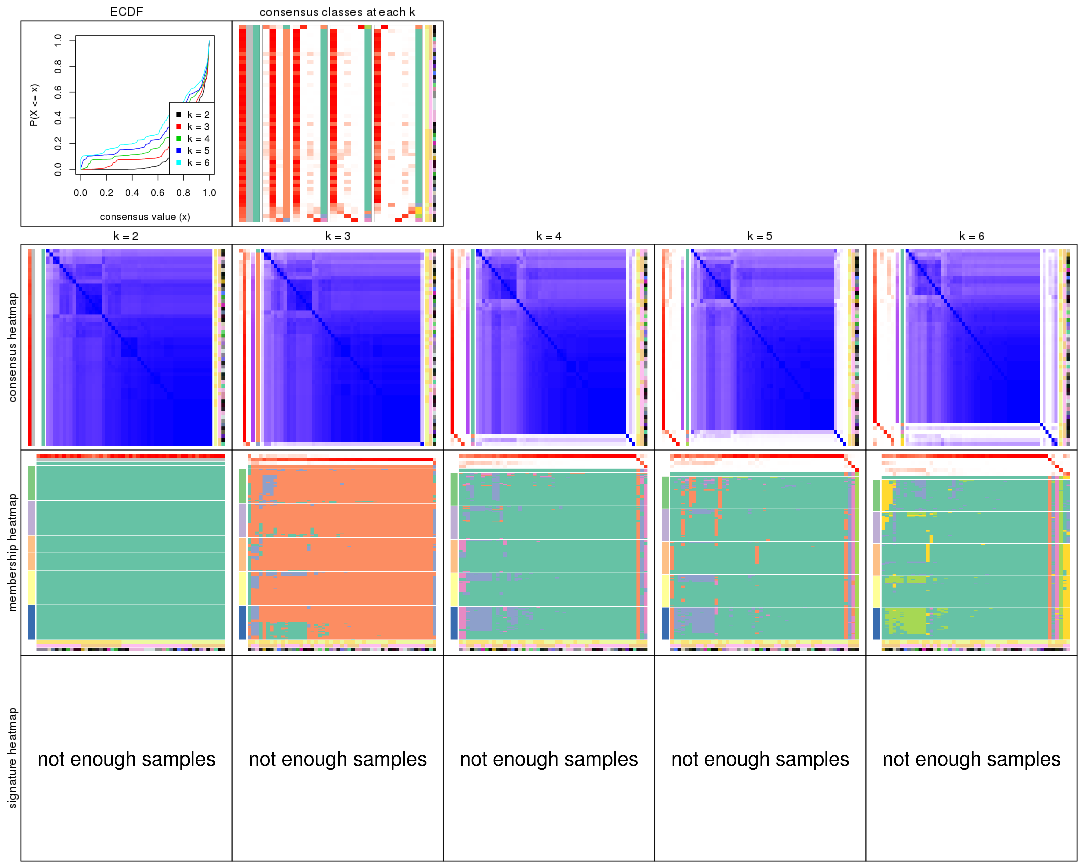
The plots are:
k and the heatmap of
predicted classes for each k.k.k.k.All the plots in panels can be made by individual functions and they are plotted later in this section.
select_partition_number() produces several plots showing different
statistics for choosing “optimized” k. There are following statistics:
k;k, the area increased is defined as \(A_k - A_{k-1}\).The detailed explanations of these statistics can be found in the cola vignette.
Generally speaking, lower PAC score, higher mean silhouette score or higher
concordance corresponds to better partition. Rand index and Jaccard index
measure how similar the current partition is compared to partition with k-1.
If they are too similar, we won't accept k is better than k-1.
select_partition_number(res)
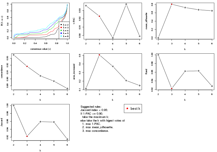
The numeric values for all these statistics can be obtained by get_stats().
get_stats(res)
#>   k 1-PAC mean_silhouette concordance area_increased  Rand Jaccard
#> 2 2 0.536           0.000       0.935          0.114 1.000   1.000
#> 3 3 0.523           0.806       0.918          0.506 0.922   0.922
#> 4 4 0.497           0.726       0.904          0.372 0.962   0.959
#> 5 5 0.537           0.674       0.897          0.207 0.963   0.958
#> 6 6 0.499           0.649       0.886          0.149 0.928   0.915
suggest_best_k() suggests the best \(k\) based on these statistics. The rules are as follows:
suggest_best_k(res)
#> [1] 3
Following shows the table of the partitions (You need to click the show/hide
code output link to see it). The membership matrix (columns with name p*)
is inferred by
clue::cl_consensus()
function with the SE method. Basically the value in the membership matrix
represents the probability to belong to a certain group. The finall class
label for an item is determined with the group with highest probability it
belongs to.
In get_classes() function, the entropy is calculated from the membership
matrix and the silhouette score is calculated from the consensus matrix.
cbind(get_classes(res, k = 2), get_membership(res, k = 2))
#>           class entropy silhouette    p1 p2
#> GSM439800     1  0.0000          0 1.000 NA
#> GSM439790     1  0.0376          0 0.996 NA
#> GSM439827     1  0.0000          0 1.000 NA
#> GSM439811     1  0.0376          0 0.996 NA
#> GSM439795     1  0.2423          0 0.960 NA
#> GSM439805     1  0.0376          0 0.996 NA
#> GSM439781     1  0.1414          0 0.980 NA
#> GSM439807     1  0.6973          0 0.812 NA
#> GSM439820     1  0.0938          0 0.988 NA
#> GSM439784     1  0.4022          0 0.920 NA
#> GSM439824     1  0.0000          0 1.000 NA
#> GSM439794     1  0.0000          0 1.000 NA
#> GSM439809     1  0.4431          0 0.908 NA
#> GSM439785     1  0.0000          0 1.000 NA
#> GSM439803     1  0.0000          0 1.000 NA
#> GSM439778     1  0.2236          0 0.964 NA
#> GSM439791     1  0.0376          0 0.996 NA
#> GSM439786     1  0.0938          0 0.988 NA
#> GSM439828     1  0.0000          0 1.000 NA
#> GSM439806     1  0.0376          0 0.996 NA
#> GSM439815     1  0.0000          0 1.000 NA
#> GSM439817     1  0.1184          0 0.984 NA
#> GSM439796     1  0.0000          0 1.000 NA
#> GSM439798     1  0.2603          0 0.956 NA
#> GSM439821     1  0.7299          0 0.796 NA
#> GSM439823     1  0.0376          0 0.996 NA
#> GSM439813     1  0.5408          0 0.876 NA
#> GSM439801     1  0.0000          0 1.000 NA
#> GSM439810     1  0.0672          0 0.992 NA
#> GSM439783     1  0.2043          0 0.968 NA
#> GSM439826     1  0.0376          0 0.996 NA
#> GSM439812     1  0.5519          0 0.872 NA
#> GSM439818     1  0.9170          0 0.668 NA
#> GSM439792     1  0.4562          0 0.904 NA
#> GSM439802     1  0.7745          0 0.772 NA
#> GSM439825     1  0.9552          0 0.624 NA
#> GSM439780     1  0.7376          0 0.792 NA
#> GSM439787     1  0.6801          0 0.820 NA
#> GSM439808     1  0.5294          0 0.880 NA
#> GSM439804     1  0.0000          0 1.000 NA
#> GSM439822     1  0.3733          0 0.928 NA
#> GSM439816     1  0.1414          0 0.980 NA
#> GSM439789     1  0.5178          0 0.884 NA
#> GSM439799     1  0.0000          0 1.000 NA
#> GSM439814     1  0.5178          0 0.884 NA
#> GSM439782     1  0.0672          0 0.992 NA
#> GSM439779     1  0.5294          0 0.880 NA
#> GSM439793     1  0.2423          0 0.960 NA
#> GSM439788     1  0.0672          0 0.992 NA
#> GSM439797     1  0.1184          0 0.984 NA
#> GSM439819     1  0.7139          0 0.804 NA
cbind(get_classes(res, k = 3), get_membership(res, k = 3))
#>           class entropy silhouette    p1    p2    p3
#> GSM439800     2  0.0000      0.907 0.000 1.000 0.000
#> GSM439790     2  0.0237      0.907 0.004 0.996 0.000
#> GSM439827     2  0.0000      0.907 0.000 1.000 0.000
#> GSM439811     2  0.0237      0.907 0.000 0.996 0.004
#> GSM439795     2  0.2636      0.868 0.048 0.932 0.020
#> GSM439805     2  0.0237      0.907 0.004 0.996 0.000
#> GSM439781     2  0.0829      0.905 0.004 0.984 0.012
#> GSM439807     2  0.6458      0.664 0.176 0.752 0.072
#> GSM439820     2  0.0661      0.904 0.004 0.988 0.008
#> GSM439784     2  0.2959      0.857 0.100 0.900 0.000
#> GSM439824     2  0.0000      0.907 0.000 1.000 0.000
#> GSM439794     2  0.0000      0.907 0.000 1.000 0.000
#> GSM439809     2  0.3349      0.849 0.108 0.888 0.004
#> GSM439785     2  0.0000      0.907 0.000 1.000 0.000
#> GSM439803     2  0.0000      0.907 0.000 1.000 0.000
#> GSM439778     2  0.1643      0.893 0.044 0.956 0.000
#> GSM439791     2  0.0237      0.907 0.000 0.996 0.004
#> GSM439786     2  0.0424      0.906 0.000 0.992 0.008
#> GSM439828     2  0.0000      0.907 0.000 1.000 0.000
#> GSM439806     2  0.0237      0.907 0.004 0.996 0.000
#> GSM439815     2  0.0000      0.907 0.000 1.000 0.000
#> GSM439817     2  0.0424      0.906 0.000 0.992 0.008
#> GSM439796     2  0.0000      0.907 0.000 1.000 0.000
#> GSM439798     2  0.1832      0.897 0.036 0.956 0.008
#> GSM439821     2  0.6579      0.294 0.020 0.652 0.328
#> GSM439823     2  0.0237      0.907 0.000 0.996 0.004
#> GSM439813     2  0.4110      0.809 0.152 0.844 0.004
#> GSM439801     2  0.0000      0.907 0.000 1.000 0.000
#> GSM439810     2  0.0424      0.907 0.008 0.992 0.000
#> GSM439783     2  0.1411      0.897 0.036 0.964 0.000
#> GSM439826     2  0.0424      0.906 0.000 0.992 0.008
#> GSM439812     2  0.4293      0.797 0.164 0.832 0.004
#> GSM439818     1  0.7728      0.000 0.640 0.276 0.084
#> GSM439792     2  0.3500      0.844 0.116 0.880 0.004
#> GSM439802     2  0.7911      0.404 0.272 0.632 0.096
#> GSM439825     3  0.5058      0.000 0.000 0.244 0.756
#> GSM439780     2  0.6586      0.647 0.216 0.728 0.056
#> GSM439787     2  0.6476      0.677 0.184 0.748 0.068
#> GSM439808     2  0.4660      0.768 0.072 0.856 0.072
#> GSM439804     2  0.0000      0.907 0.000 1.000 0.000
#> GSM439822     2  0.2772      0.849 0.004 0.916 0.080
#> GSM439816     2  0.0829      0.905 0.004 0.984 0.012
#> GSM439789     2  0.4047      0.813 0.148 0.848 0.004
#> GSM439799     2  0.0000      0.907 0.000 1.000 0.000
#> GSM439814     2  0.3879      0.812 0.152 0.848 0.000
#> GSM439782     2  0.0592      0.906 0.012 0.988 0.000
#> GSM439779     2  0.3941      0.808 0.156 0.844 0.000
#> GSM439793     2  0.2066      0.885 0.060 0.940 0.000
#> GSM439788     2  0.0424      0.907 0.008 0.992 0.000
#> GSM439797     2  0.0424      0.906 0.000 0.992 0.008
#> GSM439819     2  0.6018      0.402 0.008 0.684 0.308
cbind(get_classes(res, k = 4), get_membership(res, k = 4))
#>           class entropy silhouette    p1    p2    p3    p4
#> GSM439800     1  0.0000      0.876 1.000 0.000 0.000 0.000
#> GSM439790     1  0.0336      0.875 0.992 0.000 0.008 0.000
#> GSM439827     1  0.0000      0.876 1.000 0.000 0.000 0.000
#> GSM439811     1  0.0188      0.875 0.996 0.004 0.000 0.000
#> GSM439795     1  0.3882      0.734 0.852 0.028 0.104 0.016
#> GSM439805     1  0.0188      0.876 0.996 0.000 0.004 0.000
#> GSM439781     1  0.0967      0.871 0.976 0.004 0.016 0.004
#> GSM439807     1  0.5956      0.511 0.700 0.032 0.228 0.040
#> GSM439820     1  0.0859      0.871 0.980 0.008 0.004 0.008
#> GSM439784     1  0.3074      0.765 0.848 0.000 0.152 0.000
#> GSM439824     1  0.0000      0.876 1.000 0.000 0.000 0.000
#> GSM439794     1  0.0000      0.876 1.000 0.000 0.000 0.000
#> GSM439809     1  0.3024      0.774 0.852 0.000 0.148 0.000
#> GSM439785     1  0.0000      0.876 1.000 0.000 0.000 0.000
#> GSM439803     1  0.0000      0.876 1.000 0.000 0.000 0.000
#> GSM439778     1  0.1474      0.855 0.948 0.000 0.052 0.000
#> GSM439791     1  0.0188      0.875 0.996 0.004 0.000 0.000
#> GSM439786     1  0.0376      0.875 0.992 0.004 0.000 0.004
#> GSM439828     1  0.0000      0.876 1.000 0.000 0.000 0.000
#> GSM439806     1  0.0188      0.876 0.996 0.000 0.004 0.000
#> GSM439815     1  0.0000      0.876 1.000 0.000 0.000 0.000
#> GSM439817     1  0.0376      0.875 0.992 0.004 0.000 0.004
#> GSM439796     1  0.0000      0.876 1.000 0.000 0.000 0.000
#> GSM439798     1  0.1585      0.861 0.952 0.004 0.040 0.004
#> GSM439821     1  0.7496     -0.114 0.540 0.016 0.144 0.300
#> GSM439823     1  0.0188      0.876 0.996 0.000 0.000 0.004
#> GSM439813     1  0.4188      0.639 0.752 0.004 0.244 0.000
#> GSM439801     1  0.0000      0.876 1.000 0.000 0.000 0.000
#> GSM439810     1  0.0469      0.875 0.988 0.000 0.012 0.000
#> GSM439783     1  0.1211      0.862 0.960 0.000 0.040 0.000
#> GSM439826     1  0.0469      0.874 0.988 0.000 0.000 0.012
#> GSM439812     1  0.4522      0.598 0.728 0.004 0.264 0.004
#> GSM439818     2  0.1661      0.000 0.052 0.944 0.000 0.004
#> GSM439792     1  0.3311      0.750 0.828 0.000 0.172 0.000
#> GSM439802     3  0.4834      0.000 0.252 0.008 0.728 0.012
#> GSM439825     4  0.2011      0.000 0.080 0.000 0.000 0.920
#> GSM439780     1  0.5855      0.409 0.648 0.024 0.308 0.020
#> GSM439787     1  0.6337      0.377 0.644 0.028 0.284 0.044
#> GSM439808     1  0.4542      0.694 0.828 0.036 0.096 0.040
#> GSM439804     1  0.0000      0.876 1.000 0.000 0.000 0.000
#> GSM439822     1  0.2797      0.801 0.900 0.000 0.032 0.068
#> GSM439816     1  0.1339      0.864 0.964 0.008 0.024 0.004
#> GSM439789     1  0.4008      0.644 0.756 0.000 0.244 0.000
#> GSM439799     1  0.0000      0.876 1.000 0.000 0.000 0.000
#> GSM439814     1  0.3873      0.667 0.772 0.000 0.228 0.000
#> GSM439782     1  0.0469      0.874 0.988 0.000 0.012 0.000
#> GSM439779     1  0.3907      0.658 0.768 0.000 0.232 0.000
#> GSM439793     1  0.1867      0.841 0.928 0.000 0.072 0.000
#> GSM439788     1  0.0469      0.875 0.988 0.000 0.012 0.000
#> GSM439797     1  0.0376      0.875 0.992 0.004 0.000 0.004
#> GSM439819     1  0.6317      0.212 0.624 0.000 0.096 0.280
cbind(get_classes(res, k = 5), get_membership(res, k = 5))
#>           class entropy silhouette    p1    p2    p3    p4    p5
#> GSM439800     1  0.0703     0.8515 0.976 0.024 0.000 0.000 0.000
#> GSM439790     1  0.0290     0.8582 0.992 0.000 0.008 0.000 0.000
#> GSM439827     1  0.0404     0.8578 0.988 0.000 0.012 0.000 0.000
#> GSM439811     1  0.0162     0.8581 0.996 0.000 0.000 0.000 0.004
#> GSM439795     1  0.4836     0.2114 0.652 0.304 0.044 0.000 0.000
#> GSM439805     1  0.0162     0.8585 0.996 0.000 0.004 0.000 0.000
#> GSM439781     1  0.1243     0.8470 0.960 0.000 0.028 0.008 0.004
#> GSM439807     1  0.5435     0.4559 0.668 0.204 0.124 0.000 0.004
#> GSM439820     1  0.0798     0.8522 0.976 0.016 0.000 0.008 0.000
#> GSM439784     1  0.2930     0.7395 0.832 0.000 0.164 0.004 0.000
#> GSM439824     1  0.0000     0.8577 1.000 0.000 0.000 0.000 0.000
#> GSM439794     1  0.0162     0.8586 0.996 0.000 0.004 0.000 0.000
#> GSM439809     1  0.2690     0.7528 0.844 0.000 0.156 0.000 0.000
#> GSM439785     1  0.0000     0.8577 1.000 0.000 0.000 0.000 0.000
#> GSM439803     1  0.0000     0.8577 1.000 0.000 0.000 0.000 0.000
#> GSM439778     1  0.1270     0.8385 0.948 0.000 0.052 0.000 0.000
#> GSM439791     1  0.0162     0.8581 0.996 0.000 0.000 0.000 0.004
#> GSM439786     1  0.0613     0.8566 0.984 0.000 0.004 0.008 0.004
#> GSM439828     1  0.0000     0.8577 1.000 0.000 0.000 0.000 0.000
#> GSM439806     1  0.0162     0.8584 0.996 0.000 0.004 0.000 0.000
#> GSM439815     1  0.0162     0.8586 0.996 0.000 0.004 0.000 0.000
#> GSM439817     1  0.0324     0.8578 0.992 0.000 0.000 0.004 0.004
#> GSM439796     1  0.0000     0.8577 1.000 0.000 0.000 0.000 0.000
#> GSM439798     1  0.1365     0.8451 0.952 0.000 0.040 0.004 0.004
#> GSM439821     2  0.5883     0.0000 0.296 0.596 0.012 0.096 0.000
#> GSM439823     1  0.0162     0.8583 0.996 0.000 0.000 0.004 0.000
#> GSM439813     1  0.3957     0.5837 0.712 0.000 0.280 0.008 0.000
#> GSM439801     1  0.0000     0.8577 1.000 0.000 0.000 0.000 0.000
#> GSM439810     1  0.0404     0.8582 0.988 0.000 0.012 0.000 0.000
#> GSM439783     1  0.1043     0.8460 0.960 0.000 0.040 0.000 0.000
#> GSM439826     1  0.0162     0.8580 0.996 0.004 0.000 0.000 0.000
#> GSM439812     1  0.4088     0.5449 0.688 0.000 0.304 0.008 0.000
#> GSM439818     5  0.0324     0.0000 0.004 0.000 0.000 0.004 0.992
#> GSM439792     1  0.3300     0.7044 0.792 0.000 0.204 0.004 0.000
#> GSM439802     3  0.2199     0.0000 0.044 0.016 0.924 0.008 0.008
#> GSM439825     4  0.0609     0.0000 0.020 0.000 0.000 0.980 0.000
#> GSM439780     1  0.5663     0.4104 0.628 0.116 0.252 0.000 0.004
#> GSM439787     1  0.6495    -0.0305 0.536 0.248 0.208 0.008 0.000
#> GSM439808     1  0.3398     0.5992 0.780 0.216 0.000 0.000 0.004
#> GSM439804     1  0.0000     0.8577 1.000 0.000 0.000 0.000 0.000
#> GSM439822     1  0.3238     0.6692 0.836 0.136 0.000 0.028 0.000
#> GSM439816     1  0.1569     0.8349 0.944 0.000 0.044 0.008 0.004
#> GSM439789     1  0.3661     0.5990 0.724 0.000 0.276 0.000 0.000
#> GSM439799     1  0.0000     0.8577 1.000 0.000 0.000 0.000 0.000
#> GSM439814     1  0.3452     0.6432 0.756 0.000 0.244 0.000 0.000
#> GSM439782     1  0.0290     0.8587 0.992 0.000 0.008 0.000 0.000
#> GSM439779     1  0.3452     0.6402 0.756 0.000 0.244 0.000 0.000
#> GSM439793     1  0.1768     0.8250 0.924 0.000 0.072 0.004 0.000
#> GSM439788     1  0.0404     0.8582 0.988 0.000 0.012 0.000 0.000
#> GSM439797     1  0.0324     0.8578 0.992 0.000 0.000 0.004 0.004
#> GSM439819     1  0.5785    -0.5043 0.504 0.404 0.000 0.092 0.000
cbind(get_classes(res, k = 6), get_membership(res, k = 6))
#>           class entropy silhouette    p1 p2    p3    p4    p5    p6
#> GSM439800     1  0.2936      0.729 0.852  0 0.112 0.020 0.000 0.016
#> GSM439790     1  0.0146      0.855 0.996  0 0.000 0.000 0.004 0.000
#> GSM439827     1  0.0806      0.848 0.972  0 0.000 0.000 0.008 0.020
#> GSM439811     1  0.0260      0.855 0.992  0 0.000 0.000 0.000 0.008
#> GSM439795     3  0.5536      0.000 0.300  0 0.536 0.000 0.000 0.164
#> GSM439805     1  0.0405      0.854 0.988  0 0.000 0.000 0.004 0.008
#> GSM439781     1  0.1003      0.845 0.964  0 0.000 0.000 0.016 0.020
#> GSM439807     1  0.4968      0.369 0.632  0 0.248 0.000 0.120 0.000
#> GSM439820     1  0.1257      0.834 0.952  0 0.020 0.000 0.000 0.028
#> GSM439784     1  0.2632      0.735 0.832  0 0.000 0.000 0.164 0.004
#> GSM439824     1  0.0000      0.855 1.000  0 0.000 0.000 0.000 0.000
#> GSM439794     1  0.0146      0.856 0.996  0 0.000 0.000 0.004 0.000
#> GSM439809     1  0.2805      0.717 0.812  0 0.000 0.000 0.184 0.004
#> GSM439785     1  0.0000      0.855 1.000  0 0.000 0.000 0.000 0.000
#> GSM439803     1  0.0000      0.855 1.000  0 0.000 0.000 0.000 0.000
#> GSM439778     1  0.1141      0.836 0.948  0 0.000 0.000 0.052 0.000
#> GSM439791     1  0.0000      0.855 1.000  0 0.000 0.000 0.000 0.000
#> GSM439786     1  0.0291      0.855 0.992  0 0.000 0.000 0.004 0.004
#> GSM439828     1  0.0000      0.855 1.000  0 0.000 0.000 0.000 0.000
#> GSM439806     1  0.0146      0.855 0.996  0 0.000 0.000 0.004 0.000
#> GSM439815     1  0.0622      0.852 0.980  0 0.012 0.000 0.000 0.008
#> GSM439817     1  0.0000      0.855 1.000  0 0.000 0.000 0.000 0.000
#> GSM439796     1  0.0000      0.855 1.000  0 0.000 0.000 0.000 0.000
#> GSM439798     1  0.0937      0.844 0.960  0 0.000 0.000 0.040 0.000
#> GSM439821     6  0.2805     -0.177 0.184  0 0.004 0.000 0.000 0.812
#> GSM439823     1  0.0146      0.855 0.996  0 0.000 0.000 0.000 0.004
#> GSM439813     1  0.4504      0.468 0.648  0 0.012 0.000 0.308 0.032
#> GSM439801     1  0.0000      0.855 1.000  0 0.000 0.000 0.000 0.000
#> GSM439810     1  0.0260      0.856 0.992  0 0.000 0.000 0.008 0.000
#> GSM439783     1  0.0937      0.843 0.960  0 0.000 0.000 0.040 0.000
#> GSM439826     1  0.0146      0.855 0.996  0 0.000 0.000 0.000 0.004
#> GSM439812     1  0.4855      0.408 0.616  0 0.012 0.000 0.320 0.052
#> GSM439818     2  0.0000      0.000 0.000  1 0.000 0.000 0.000 0.000
#> GSM439792     1  0.3709      0.655 0.756  0 0.000 0.000 0.204 0.040
#> GSM439802     5  0.2257      0.000 0.004  0 0.028 0.004 0.904 0.060
#> GSM439825     4  0.0632      0.000 0.000  0 0.000 0.976 0.000 0.024
#> GSM439780     1  0.5116      0.385 0.612  0 0.132 0.000 0.256 0.000
#> GSM439787     1  0.6730     -0.199 0.496  0 0.084 0.000 0.176 0.244
#> GSM439808     1  0.3515      0.348 0.676  0 0.324 0.000 0.000 0.000
#> GSM439804     1  0.0000      0.855 1.000  0 0.000 0.000 0.000 0.000
#> GSM439822     1  0.2772      0.622 0.816  0 0.004 0.000 0.000 0.180
#> GSM439816     1  0.2250      0.791 0.896  0 0.000 0.000 0.064 0.040
#> GSM439789     1  0.3835      0.531 0.684  0 0.000 0.000 0.300 0.016
#> GSM439799     1  0.0000      0.855 1.000  0 0.000 0.000 0.000 0.000
#> GSM439814     1  0.3445      0.604 0.732  0 0.008 0.000 0.260 0.000
#> GSM439782     1  0.0260      0.856 0.992  0 0.000 0.000 0.008 0.000
#> GSM439779     1  0.3151      0.624 0.748  0 0.000 0.000 0.252 0.000
#> GSM439793     1  0.1644      0.820 0.920  0 0.000 0.000 0.076 0.004
#> GSM439788     1  0.0363      0.855 0.988  0 0.000 0.000 0.012 0.000
#> GSM439797     1  0.0000      0.855 1.000  0 0.000 0.000 0.000 0.000
#> GSM439819     6  0.3961     -0.037 0.440  0 0.004 0.000 0.000 0.556
Heatmaps for the consensus matrix. It visualizes the probability of two samples to be in a same group.
consensus_heatmap(res, k = 2)
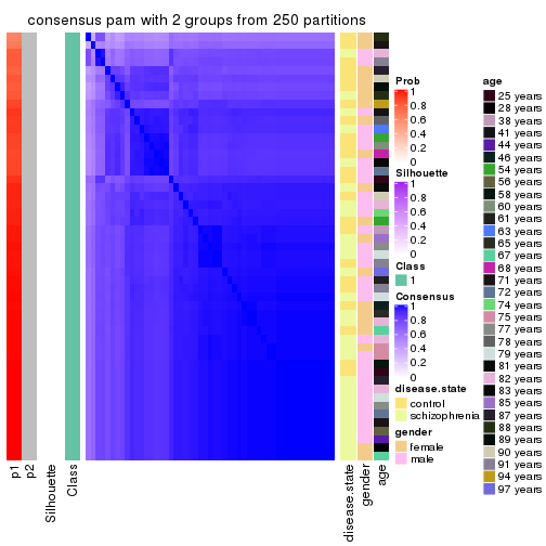
consensus_heatmap(res, k = 3)
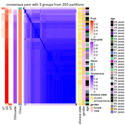
consensus_heatmap(res, k = 4)
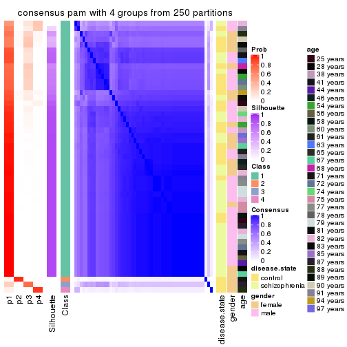
consensus_heatmap(res, k = 5)
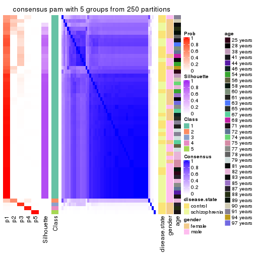
consensus_heatmap(res, k = 6)
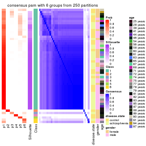
Heatmaps for the membership of samples in all partitions to see how consistent they are:
membership_heatmap(res, k = 2)
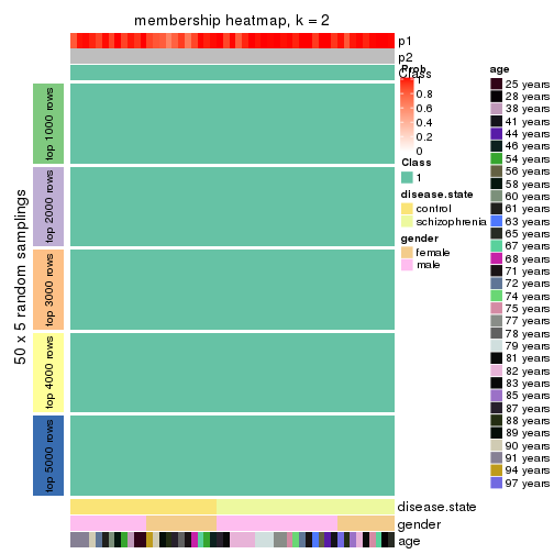
membership_heatmap(res, k = 3)
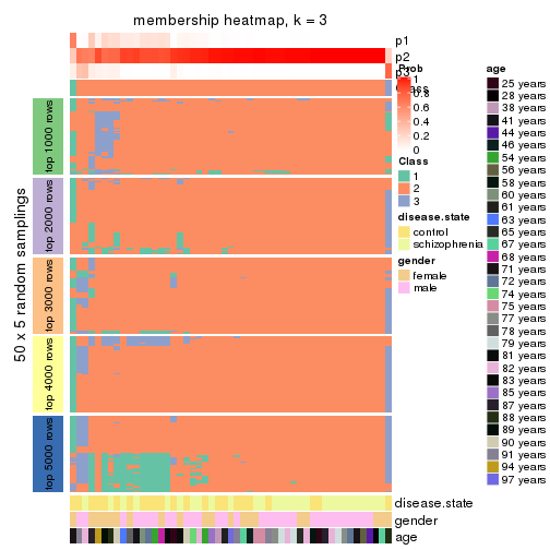
membership_heatmap(res, k = 4)
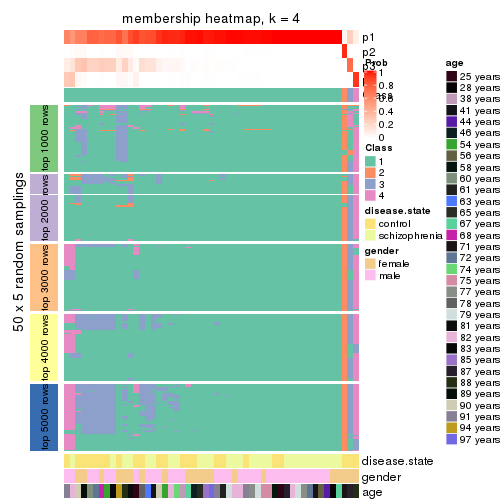
membership_heatmap(res, k = 5)
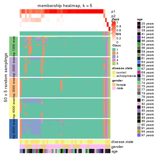
membership_heatmap(res, k = 6)
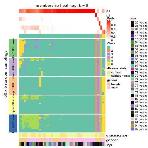
As soon as we have had the classes for columns, we can look for signatures which are significantly different between classes which can be candidate marks for certain classes. Following are the heatmaps for signatures.
Signature heatmaps where rows are scaled:
get_signatures(res, k = 2)

get_signatures(res, k = 3)

get_signatures(res, k = 4)

get_signatures(res, k = 5)

get_signatures(res, k = 6)

Signature heatmaps where rows are not scaled:
get_signatures(res, k = 2, scale_rows = FALSE)

get_signatures(res, k = 3, scale_rows = FALSE)

get_signatures(res, k = 4, scale_rows = FALSE)

get_signatures(res, k = 5, scale_rows = FALSE)

get_signatures(res, k = 6, scale_rows = FALSE)

Compare the overlap of signatures from different k:
compare_signatures(res)
get_signature() returns a data frame invisibly. TO get the list of signatures, the function
call should be assigned to a variable explicitly. In following code, if plot argument is set
to FALSE, no heatmap is plotted while only the differential analysis is performed.
# code only for demonstration
tb = get_signature(res, k = ..., plot = FALSE)
An example of the output of tb is:
#>   which_row         fdr    mean_1    mean_2 scaled_mean_1 scaled_mean_2 km
#> 1        38 0.042760348  8.373488  9.131774    -0.5533452     0.5164555  1
#> 2        40 0.018707592  7.106213  8.469186    -0.6173731     0.5762149  1
#> 3        55 0.019134737 10.221463 11.207825    -0.6159697     0.5749050  1
#> 4        59 0.006059896  5.921854  7.869574    -0.6899429     0.6439467  1
#> 5        60 0.018055526  8.928898 10.211722    -0.6204761     0.5791110  1
#> 6        98 0.009384629 15.714769 14.887706     0.6635654    -0.6193277  2
...
The columns in tb are:
which_row: row indices corresponding to the input matrix.fdr: FDR for the differential test. mean_x: The mean value in group x.scaled_mean_x: The mean value in group x after rows are scaled.km: Row groups if k-means clustering is applied to rows.UMAP plot which shows how samples are separated.
dimension_reduction(res, k = 2, method = "UMAP")
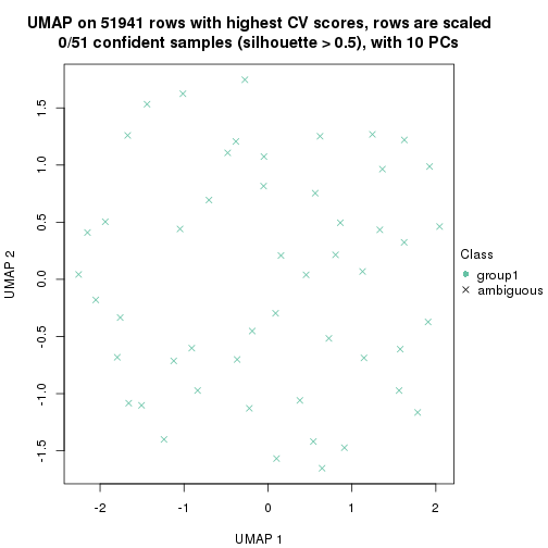
dimension_reduction(res, k = 3, method = "UMAP")
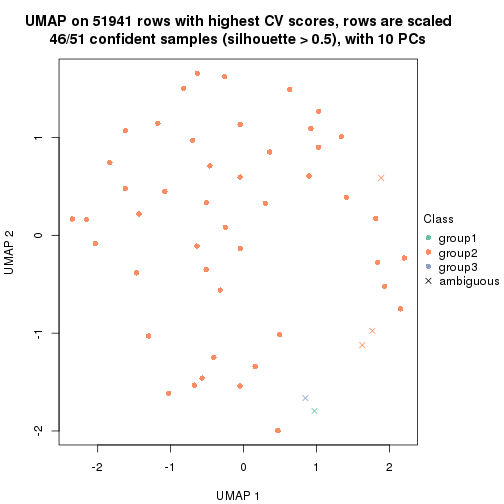
dimension_reduction(res, k = 4, method = "UMAP")
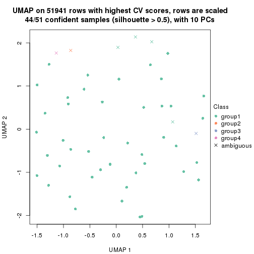
dimension_reduction(res, k = 5, method = "UMAP")
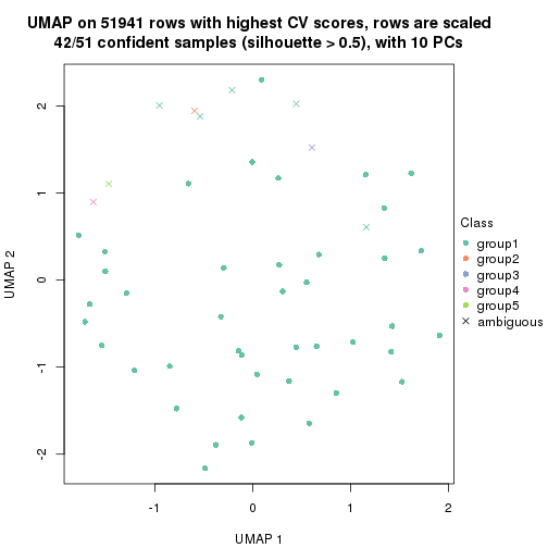
dimension_reduction(res, k = 6, method = "UMAP")
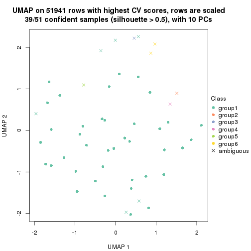
Following heatmap shows how subgroups are split when increasing k:
collect_classes(res)
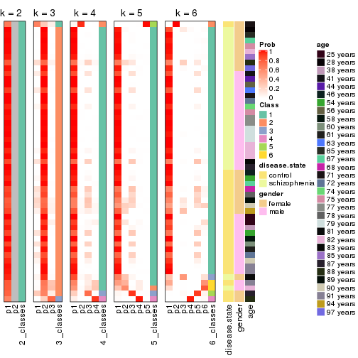
Test correlation between subgroups and known annotations. If the known annotation is numeric, one-way ANOVA test is applied, and if the known annotation is discrete, chi-squared contingency table test is applied.
test_to_known_factors(res)
#>         n disease.state(p) gender(p) age(p) k
#> CV:pam  0               NA        NA     NA 2
#> CV:pam 46               NA        NA     NA 3
#> CV:pam 44               NA        NA     NA 4
#> CV:pam 42               NA        NA     NA 5
#> CV:pam 39               NA        NA     NA 6
If matrix rows can be associated to genes, consider to use functional_enrichment(res,
...) to perform function enrichment for the signature genes. See this vignette for more detailed explanations.
The object with results only for a single top-value method and a single partition method can be extracted as:
res = res_list["CV", "mclust"]
# you can also extract it by
# res = res_list["CV:mclust"]
A summary of res and all the functions that can be applied to it:
res
#> A 'ConsensusPartition' object with k = 2, 3, 4, 5, 6.
#>   On a matrix with 51941 rows and 51 columns.
#>   Top rows (1000, 2000, 3000, 4000, 5000) are extracted by 'CV' method.
#>   Subgroups are detected by 'mclust' method.
#>   Performed in total 1250 partitions by row resampling.
#>   Best k for subgroups seems to be 2.
#>
#> Following methods can be applied to this 'ConsensusPartition' object:
#>  [1] "cola_report"             "collect_classes"         "collect_plots"
#>  [4] "collect_stats"           "colnames"                "compare_signatures"
#>  [7] "consensus_heatmap"       "dimension_reduction"     "functional_enrichment"
#> [10] "get_anno_col"            "get_anno"                "get_classes"
#> [13] "get_consensus"           "get_matrix"              "get_membership"
#> [16] "get_param"               "get_signatures"          "get_stats"
#> [19] "is_best_k"               "is_stable_k"             "membership_heatmap"
#> [22] "ncol"                    "nrow"                    "plot_ecdf"
#> [25] "rownames"                "select_partition_number" "show"
#> [28] "suggest_best_k"          "test_to_known_factors"
collect_plots() function collects all the plots made from res for all k (number of partitions)
into one single page to provide an easy and fast comparison between different k.
collect_plots(res)
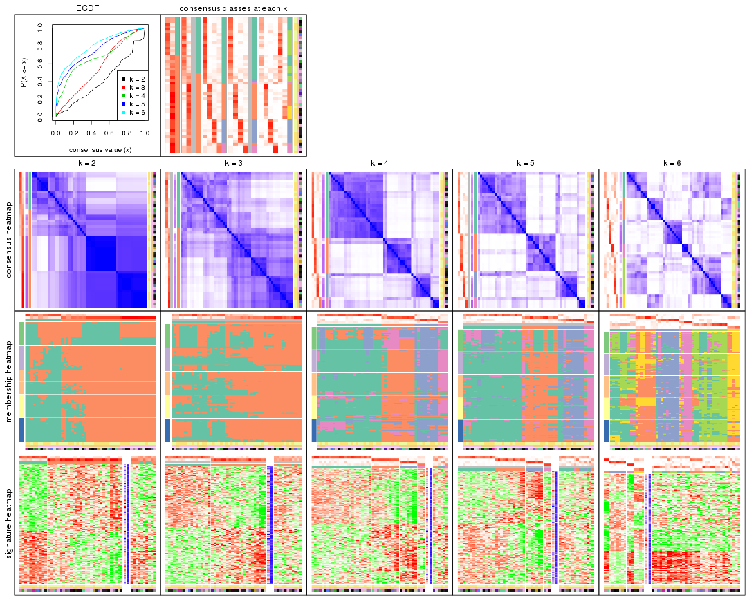
The plots are:
k and the heatmap of
predicted classes for each k.k.k.k.All the plots in panels can be made by individual functions and they are plotted later in this section.
select_partition_number() produces several plots showing different
statistics for choosing “optimized” k. There are following statistics:
k;k, the area increased is defined as \(A_k - A_{k-1}\).The detailed explanations of these statistics can be found in the cola vignette.
Generally speaking, lower PAC score, higher mean silhouette score or higher
concordance corresponds to better partition. Rand index and Jaccard index
measure how similar the current partition is compared to partition with k-1.
If they are too similar, we won't accept k is better than k-1.
select_partition_number(res)
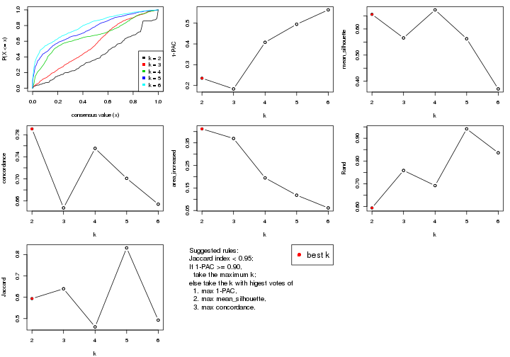
The numeric values for all these statistics can be obtained by get_stats().
get_stats(res)
#>   k 1-PAC mean_silhouette concordance area_increased  Rand Jaccard
#> 2 2 0.235           0.656       0.791         0.4118 0.594   0.594
#> 3 3 0.184           0.566       0.647         0.3694 0.758   0.640
#> 4 4 0.408           0.673       0.755         0.1945 0.692   0.461
#> 5 5 0.495           0.563       0.701         0.1179 0.941   0.831
#> 6 6 0.564           0.371       0.654         0.0616 0.836   0.493
suggest_best_k() suggests the best \(k\) based on these statistics. The rules are as follows:
suggest_best_k(res)
#> [1] 2
Following shows the table of the partitions (You need to click the show/hide
code output link to see it). The membership matrix (columns with name p*)
is inferred by
clue::cl_consensus()
function with the SE method. Basically the value in the membership matrix
represents the probability to belong to a certain group. The finall class
label for an item is determined with the group with highest probability it
belongs to.
In get_classes() function, the entropy is calculated from the membership
matrix and the silhouette score is calculated from the consensus matrix.
cbind(get_classes(res, k = 2), get_membership(res, k = 2))
#>           class entropy silhouette    p1    p2
#> GSM439800     2  0.5629      0.785 0.132 0.868
#> GSM439790     1  0.9580      0.343 0.620 0.380
#> GSM439827     2  0.5408      0.785 0.124 0.876
#> GSM439811     2  0.5408      0.785 0.124 0.876
#> GSM439795     2  0.5408      0.785 0.124 0.876
#> GSM439805     2  0.5519      0.786 0.128 0.872
#> GSM439781     2  0.8661      0.647 0.288 0.712
#> GSM439807     2  0.5519      0.786 0.128 0.872
#> GSM439820     2  0.5408      0.785 0.124 0.876
#> GSM439784     2  0.8443      0.455 0.272 0.728
#> GSM439824     2  0.0376      0.799 0.004 0.996
#> GSM439794     2  0.0672      0.797 0.008 0.992
#> GSM439809     1  0.6148      0.758 0.848 0.152
#> GSM439785     2  0.8763      0.370 0.296 0.704
#> GSM439803     2  0.0938      0.797 0.012 0.988
#> GSM439778     1  0.9977      0.445 0.528 0.472
#> GSM439791     1  0.5629      0.752 0.868 0.132
#> GSM439786     2  0.9954     -0.281 0.460 0.540
#> GSM439828     2  0.0000      0.799 0.000 1.000
#> GSM439806     1  0.5629      0.752 0.868 0.132
#> GSM439815     2  0.8608      0.398 0.284 0.716
#> GSM439817     2  0.0672      0.797 0.008 0.992
#> GSM439796     2  0.0938      0.797 0.012 0.988
#> GSM439798     2  0.8144      0.501 0.252 0.748
#> GSM439821     2  0.0000      0.799 0.000 1.000
#> GSM439823     2  0.0000      0.799 0.000 1.000
#> GSM439813     1  0.9954      0.438 0.540 0.460
#> GSM439801     2  0.0938      0.797 0.012 0.988
#> GSM439810     1  0.4562      0.713 0.904 0.096
#> GSM439783     1  0.8081      0.624 0.752 0.248
#> GSM439826     2  0.5408      0.785 0.124 0.876
#> GSM439812     1  0.3733      0.710 0.928 0.072
#> GSM439818     2  0.5408      0.785 0.124 0.876
#> GSM439792     1  0.8081      0.619 0.752 0.248
#> GSM439802     2  0.5629      0.785 0.132 0.868
#> GSM439825     2  0.5408      0.785 0.124 0.876
#> GSM439780     2  0.9248      0.553 0.340 0.660
#> GSM439787     2  0.5408      0.785 0.124 0.876
#> GSM439808     2  0.5408      0.785 0.124 0.876
#> GSM439804     2  0.0938      0.797 0.012 0.988
#> GSM439822     2  0.0000      0.799 0.000 1.000
#> GSM439816     2  0.2778      0.774 0.048 0.952
#> GSM439789     2  0.9963     -0.264 0.464 0.536
#> GSM439799     2  0.0000      0.799 0.000 1.000
#> GSM439814     1  0.8813      0.702 0.700 0.300
#> GSM439782     2  0.9209      0.219 0.336 0.664
#> GSM439779     1  0.5519      0.750 0.872 0.128
#> GSM439793     1  0.8661      0.717 0.712 0.288
#> GSM439788     1  0.6712      0.759 0.824 0.176
#> GSM439797     2  0.8499      0.416 0.276 0.724
#> GSM439819     2  0.0000      0.799 0.000 1.000
cbind(get_classes(res, k = 3), get_membership(res, k = 3))
#>           class entropy silhouette    p1    p2 p3
#> GSM439800     2  0.7344     0.6256 0.084 0.684 NA
#> GSM439790     1  0.8626     0.5091 0.580 0.280 NA
#> GSM439827     2  0.1163     0.6751 0.000 0.972 NA
#> GSM439811     2  0.1163     0.6751 0.000 0.972 NA
#> GSM439795     2  0.6255     0.6223 0.012 0.668 NA
#> GSM439805     2  0.7259     0.6249 0.072 0.680 NA
#> GSM439781     2  0.9738     0.0213 0.264 0.448 NA
#> GSM439807     2  0.7056     0.6157 0.044 0.656 NA
#> GSM439820     2  0.0829     0.6806 0.004 0.984 NA
#> GSM439784     1  0.9225     0.4638 0.532 0.256 NA
#> GSM439824     2  0.6771     0.5571 0.276 0.684 NA
#> GSM439794     2  0.8491     0.4640 0.312 0.572 NA
#> GSM439809     1  0.6357     0.6493 0.684 0.020 NA
#> GSM439785     1  0.9050     0.0593 0.484 0.376 NA
#> GSM439803     2  0.9527     0.3586 0.300 0.480 NA
#> GSM439778     1  0.6726     0.6668 0.748 0.120 NA
#> GSM439791     1  0.2590     0.6789 0.924 0.004 NA
#> GSM439786     1  0.8293     0.6457 0.608 0.120 NA
#> GSM439828     2  0.4479     0.6575 0.044 0.860 NA
#> GSM439806     1  0.5728     0.6564 0.720 0.008 NA
#> GSM439815     1  0.7898     0.6047 0.652 0.116 NA
#> GSM439817     2  0.6255     0.6172 0.204 0.748 NA
#> GSM439796     2  0.9347     0.4233 0.276 0.512 NA
#> GSM439798     1  0.9702     0.4252 0.444 0.236 NA
#> GSM439821     2  0.4589     0.6359 0.008 0.820 NA
#> GSM439823     2  0.5000     0.6634 0.044 0.832 NA
#> GSM439813     1  0.5961     0.6718 0.788 0.076 NA
#> GSM439801     2  0.8566     0.5883 0.188 0.608 NA
#> GSM439810     1  0.6425     0.6243 0.764 0.140 NA
#> GSM439783     1  0.7344     0.5947 0.680 0.240 NA
#> GSM439826     2  0.2261     0.6553 0.000 0.932 NA
#> GSM439812     1  0.6910     0.6186 0.736 0.144 NA
#> GSM439818     2  0.2356     0.6554 0.000 0.928 NA
#> GSM439792     1  0.9680     0.5485 0.456 0.244 NA
#> GSM439802     2  0.6742     0.6156 0.028 0.656 NA
#> GSM439825     2  0.2537     0.6501 0.000 0.920 NA
#> GSM439780     2  0.9383     0.0846 0.364 0.460 NA
#> GSM439787     2  0.5698     0.6518 0.012 0.736 NA
#> GSM439808     2  0.5122     0.6670 0.012 0.788 NA
#> GSM439804     2  0.9391     0.4012 0.284 0.504 NA
#> GSM439822     2  0.4748     0.6406 0.024 0.832 NA
#> GSM439816     2  0.7492     0.4669 0.340 0.608 NA
#> GSM439789     1  0.6243     0.6560 0.776 0.124 NA
#> GSM439799     2  0.6174     0.6701 0.064 0.768 NA
#> GSM439814     1  0.3009     0.6960 0.920 0.052 NA
#> GSM439782     1  0.7843     0.6125 0.664 0.128 NA
#> GSM439779     1  0.5517     0.6539 0.728 0.004 NA
#> GSM439793     1  0.7525     0.6614 0.676 0.096 NA
#> GSM439788     1  0.5731     0.6735 0.752 0.020 NA
#> GSM439797     2  0.8135     0.1773 0.448 0.484 NA
#> GSM439819     2  0.4741     0.6371 0.020 0.828 NA
cbind(get_classes(res, k = 4), get_membership(res, k = 4))
#>           class entropy silhouette    p1    p2    p3    p4
#> GSM439800     3   0.534     0.6333 0.036 0.044 0.772 0.148
#> GSM439790     1   0.516     0.6243 0.708 0.012 0.264 0.016
#> GSM439827     2   0.334     0.7475 0.008 0.880 0.080 0.032
#> GSM439811     2   0.334     0.7465 0.008 0.880 0.080 0.032
#> GSM439795     3   0.189     0.7377 0.016 0.044 0.940 0.000
#> GSM439805     3   0.258     0.7407 0.052 0.036 0.912 0.000
#> GSM439781     1   0.715     0.5881 0.600 0.032 0.276 0.092
#> GSM439807     3   0.183     0.7405 0.032 0.024 0.944 0.000
#> GSM439820     2   0.474     0.7395 0.012 0.800 0.136 0.052
#> GSM439784     1   0.326     0.7875 0.872 0.012 0.008 0.108
#> GSM439824     2   0.834     0.0871 0.372 0.444 0.060 0.124
#> GSM439794     1   0.855     0.1422 0.524 0.120 0.116 0.240
#> GSM439809     1   0.390     0.7758 0.824 0.008 0.012 0.156
#> GSM439785     1   0.528     0.7154 0.792 0.056 0.056 0.096
#> GSM439803     4   0.697     0.7999 0.184 0.068 0.080 0.668
#> GSM439778     1   0.255     0.7902 0.916 0.004 0.024 0.056
#> GSM439791     1   0.231     0.7891 0.924 0.000 0.032 0.044
#> GSM439786     1   0.516     0.7558 0.756 0.008 0.052 0.184
#> GSM439828     2   0.395     0.7524 0.020 0.848 0.024 0.108
#> GSM439806     1   0.325     0.7804 0.852 0.000 0.008 0.140
#> GSM439815     1   0.405     0.7468 0.824 0.004 0.028 0.144
#> GSM439817     2   0.739     0.4048 0.240 0.612 0.056 0.092
#> GSM439796     4   0.696     0.8132 0.164 0.076 0.084 0.676
#> GSM439798     1   0.607     0.7297 0.712 0.016 0.100 0.172
#> GSM439821     2   0.493     0.7432 0.012 0.792 0.068 0.128
#> GSM439823     2   0.462     0.7406 0.016 0.804 0.036 0.144
#> GSM439813     1   0.162     0.7922 0.952 0.000 0.020 0.028
#> GSM439801     3   0.807     0.1754 0.136 0.092 0.584 0.188
#> GSM439810     1   0.523     0.6970 0.740 0.012 0.212 0.036
#> GSM439783     1   0.463     0.7122 0.776 0.024 0.192 0.008
#> GSM439826     2   0.212     0.7707 0.008 0.924 0.068 0.000
#> GSM439812     1   0.555     0.7064 0.740 0.020 0.188 0.052
#> GSM439818     2   0.388     0.7475 0.004 0.840 0.124 0.032
#> GSM439792     1   0.659     0.7090 0.680 0.024 0.172 0.124
#> GSM439802     3   0.265     0.7372 0.056 0.028 0.912 0.004
#> GSM439825     2   0.359     0.7547 0.004 0.860 0.104 0.032
#> GSM439780     3   0.620    -0.1800 0.472 0.016 0.488 0.024
#> GSM439787     3   0.268     0.7217 0.012 0.092 0.896 0.000
#> GSM439808     3   0.440     0.6366 0.016 0.168 0.800 0.016
#> GSM439804     4   0.694     0.8138 0.168 0.072 0.084 0.676
#> GSM439822     2   0.366     0.7546 0.016 0.864 0.024 0.096
#> GSM439816     1   0.587     0.6467 0.748 0.136 0.076 0.040
#> GSM439789     1   0.159     0.7932 0.956 0.008 0.008 0.028
#> GSM439799     4   0.711     0.3251 0.024 0.292 0.096 0.588
#> GSM439814     1   0.185     0.7916 0.948 0.008 0.020 0.024
#> GSM439782     1   0.352     0.7707 0.856 0.000 0.032 0.112
#> GSM439779     1   0.330     0.7812 0.848 0.000 0.008 0.144
#> GSM439793     1   0.296     0.7855 0.876 0.004 0.004 0.116
#> GSM439788     1   0.259     0.7864 0.884 0.000 0.000 0.116
#> GSM439797     1   0.553     0.6964 0.780 0.080 0.060 0.080
#> GSM439819     2   0.468     0.7452 0.012 0.808 0.060 0.120
cbind(get_classes(res, k = 5), get_membership(res, k = 5))
#>           class entropy silhouette    p1    p2    p3    p4 p5
#> GSM439800     3   0.443    0.64294 0.016 0.036 0.796 0.132 NA
#> GSM439790     1   0.654    0.45255 0.536 0.000 0.264 0.012 NA
#> GSM439827     2   0.558    0.67692 0.000 0.680 0.040 0.064 NA
#> GSM439811     2   0.551    0.67834 0.000 0.684 0.036 0.064 NA
#> GSM439795     3   0.148    0.71137 0.000 0.048 0.944 0.000 NA
#> GSM439805     3   0.204    0.71672 0.008 0.036 0.932 0.016 NA
#> GSM439781     3   0.726   -0.22444 0.300 0.012 0.364 0.004 NA
#> GSM439807     3   0.209    0.71678 0.024 0.024 0.932 0.008 NA
#> GSM439820     2   0.659    0.68377 0.000 0.580 0.116 0.048 NA
#> GSM439784     1   0.579    0.58251 0.612 0.040 0.028 0.008 NA
#> GSM439824     2   0.579    0.53676 0.128 0.720 0.016 0.064 NA
#> GSM439794     4   0.830    0.25506 0.304 0.232 0.088 0.364 NA
#> GSM439809     1   0.567    0.58105 0.576 0.016 0.000 0.056 NA
#> GSM439785     1   0.584    0.45611 0.680 0.040 0.016 0.212 NA
#> GSM439803     4   0.255    0.79799 0.080 0.016 0.004 0.896 NA
#> GSM439778     1   0.453    0.58635 0.780 0.000 0.032 0.052 NA
#> GSM439791     1   0.215    0.63533 0.924 0.004 0.004 0.028 NA
#> GSM439786     1   0.787    0.49731 0.500 0.008 0.136 0.152 NA
#> GSM439828     2   0.120    0.71241 0.000 0.960 0.004 0.004 NA
#> GSM439806     1   0.456    0.61261 0.676 0.000 0.000 0.032 NA
#> GSM439815     1   0.633    0.46781 0.620 0.000 0.036 0.196 NA
#> GSM439817     2   0.595    0.49436 0.132 0.692 0.012 0.128 NA
#> GSM439796     4   0.221    0.79766 0.072 0.020 0.000 0.908 NA
#> GSM439798     1   0.825    0.44728 0.400 0.008 0.172 0.124 NA
#> GSM439821     2   0.475    0.67732 0.000 0.756 0.084 0.016 NA
#> GSM439823     2   0.143    0.70972 0.000 0.944 0.004 0.052 NA
#> GSM439813     1   0.456    0.58302 0.768 0.000 0.028 0.044 NA
#> GSM439801     3   0.662    0.30141 0.056 0.104 0.600 0.236 NA
#> GSM439810     1   0.506    0.58466 0.732 0.000 0.140 0.016 NA
#> GSM439783     1   0.474    0.59223 0.748 0.000 0.148 0.008 NA
#> GSM439826     2   0.418    0.72204 0.004 0.792 0.016 0.032 NA
#> GSM439812     1   0.526    0.58010 0.708 0.000 0.128 0.012 NA
#> GSM439818     2   0.652    0.67551 0.000 0.580 0.104 0.048 NA
#> GSM439792     1   0.629    0.48467 0.448 0.000 0.152 0.000 NA
#> GSM439802     3   0.253    0.70978 0.040 0.024 0.912 0.008 NA
#> GSM439825     2   0.642    0.67848 0.000 0.588 0.100 0.044 NA
#> GSM439780     3   0.637    0.00156 0.368 0.000 0.512 0.024 NA
#> GSM439787     3   0.250    0.70434 0.000 0.064 0.900 0.004 NA
#> GSM439808     3   0.405    0.58054 0.000 0.180 0.780 0.008 NA
#> GSM439804     4   0.223    0.79866 0.080 0.016 0.000 0.904 NA
#> GSM439822     2   0.161    0.71768 0.000 0.928 0.000 0.000 NA
#> GSM439816     1   0.754    0.13972 0.504 0.296 0.028 0.120 NA
#> GSM439789     1   0.358    0.60344 0.852 0.012 0.008 0.048 NA
#> GSM439799     2   0.685    0.29599 0.000 0.492 0.108 0.352 NA
#> GSM439814     1   0.216    0.63244 0.924 0.004 0.012 0.012 NA
#> GSM439782     1   0.589    0.51696 0.664 0.000 0.028 0.152 NA
#> GSM439779     1   0.415    0.61157 0.676 0.000 0.000 0.008 NA
#> GSM439793     1   0.499    0.58900 0.624 0.004 0.016 0.012 NA
#> GSM439788     1   0.445    0.60396 0.660 0.000 0.008 0.008 NA
#> GSM439797     1   0.676    0.38876 0.620 0.120 0.024 0.196 NA
#> GSM439819     2   0.433    0.69133 0.000 0.784 0.056 0.016 NA
cbind(get_classes(res, k = 6), get_membership(res, k = 6))
#>           class entropy silhouette    p1    p2    p3    p4    p5    p6
#> GSM439800     3  0.4015    0.67632 0.036 0.012 0.772 0.172 0.004 0.004
#> GSM439790     5  0.7038    0.01760 0.344 0.000 0.224 0.004 0.368 0.060
#> GSM439827     2  0.0665    0.52842 0.008 0.980 0.008 0.004 0.000 0.000
#> GSM439811     2  0.0665    0.52842 0.008 0.980 0.008 0.004 0.000 0.000
#> GSM439795     3  0.1026    0.77620 0.008 0.012 0.968 0.000 0.004 0.008
#> GSM439805     3  0.1026    0.77814 0.008 0.004 0.968 0.012 0.008 0.000
#> GSM439781     5  0.6377    0.24663 0.180 0.008 0.212 0.004 0.560 0.036
#> GSM439807     3  0.1708    0.77554 0.024 0.000 0.932 0.000 0.040 0.004
#> GSM439820     2  0.5229   -0.01286 0.004 0.656 0.096 0.020 0.000 0.224
#> GSM439784     5  0.2781    0.41144 0.016 0.060 0.012 0.008 0.888 0.016
#> GSM439824     2  0.6492    0.45898 0.068 0.640 0.004 0.112 0.084 0.092
#> GSM439794     4  0.7669    0.32548 0.088 0.216 0.056 0.488 0.144 0.008
#> GSM439809     5  0.3593    0.40416 0.100 0.000 0.004 0.052 0.824 0.020
#> GSM439785     1  0.7715    0.22008 0.368 0.096 0.008 0.240 0.276 0.012
#> GSM439803     4  0.1381    0.70932 0.020 0.000 0.004 0.952 0.020 0.004
#> GSM439778     1  0.6238    0.33207 0.448 0.000 0.004 0.020 0.372 0.156
#> GSM439791     5  0.4076   -0.07497 0.348 0.000 0.000 0.004 0.636 0.012
#> GSM439786     5  0.8225    0.00923 0.236 0.000 0.148 0.168 0.380 0.068
#> GSM439828     2  0.4178    0.36028 0.004 0.660 0.004 0.016 0.000 0.316
#> GSM439806     5  0.2737    0.40232 0.096 0.000 0.000 0.024 0.868 0.012
#> GSM439815     1  0.7272    0.32912 0.468 0.000 0.008 0.168 0.208 0.148
#> GSM439817     2  0.6030    0.45521 0.024 0.660 0.008 0.152 0.100 0.056
#> GSM439796     4  0.0858    0.71294 0.000 0.000 0.000 0.968 0.028 0.004
#> GSM439798     5  0.6956    0.20683 0.152 0.000 0.160 0.100 0.556 0.032
#> GSM439821     6  0.3933    0.67475 0.004 0.216 0.040 0.000 0.000 0.740
#> GSM439823     2  0.4727    0.27763 0.004 0.600 0.004 0.040 0.000 0.352
#> GSM439813     1  0.5735    0.31487 0.444 0.000 0.000 0.000 0.388 0.168
#> GSM439801     3  0.5304    0.42742 0.028 0.028 0.636 0.284 0.016 0.008
#> GSM439810     1  0.5087    0.11455 0.500 0.000 0.044 0.000 0.440 0.016
#> GSM439783     1  0.5385    0.05925 0.472 0.008 0.060 0.004 0.452 0.004
#> GSM439826     2  0.3560    0.33772 0.012 0.772 0.004 0.008 0.000 0.204
#> GSM439812     1  0.5298    0.06716 0.476 0.000 0.044 0.004 0.456 0.020
#> GSM439818     6  0.4660    0.59623 0.000 0.416 0.044 0.000 0.000 0.540
#> GSM439792     5  0.4616    0.31698 0.196 0.008 0.048 0.000 0.724 0.024
#> GSM439802     3  0.3123    0.74839 0.100 0.000 0.848 0.004 0.040 0.008
#> GSM439825     6  0.4709    0.62176 0.004 0.400 0.040 0.000 0.000 0.556
#> GSM439780     3  0.6782    0.07836 0.372 0.000 0.404 0.000 0.144 0.080
#> GSM439787     3  0.2216    0.76240 0.024 0.052 0.908 0.000 0.000 0.016
#> GSM439808     3  0.3444    0.69863 0.008 0.120 0.828 0.020 0.000 0.024
#> GSM439804     4  0.0777    0.71343 0.000 0.000 0.000 0.972 0.024 0.004
#> GSM439822     6  0.4189    0.20875 0.004 0.436 0.000 0.008 0.000 0.552
#> GSM439816     5  0.8169   -0.20336 0.252 0.204 0.008 0.180 0.336 0.020
#> GSM439789     1  0.5539    0.27264 0.508 0.040 0.004 0.032 0.412 0.004
#> GSM439799     4  0.7019   -0.04404 0.000 0.176 0.076 0.452 0.008 0.288
#> GSM439814     5  0.4651   -0.14379 0.372 0.028 0.000 0.000 0.588 0.012
#> GSM439782     1  0.6692    0.33249 0.488 0.000 0.004 0.060 0.276 0.172
#> GSM439779     5  0.2212    0.37305 0.112 0.000 0.000 0.000 0.880 0.008
#> GSM439793     5  0.1414    0.43350 0.020 0.012 0.000 0.004 0.952 0.012
#> GSM439788     5  0.1363    0.43163 0.028 0.004 0.000 0.004 0.952 0.012
#> GSM439797     1  0.7835    0.17545 0.332 0.112 0.008 0.232 0.304 0.012
#> GSM439819     6  0.3807    0.67645 0.004 0.228 0.028 0.000 0.000 0.740
Heatmaps for the consensus matrix. It visualizes the probability of two samples to be in a same group.
consensus_heatmap(res, k = 2)
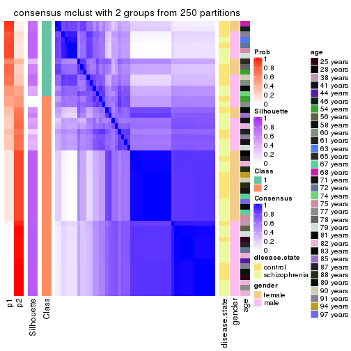
consensus_heatmap(res, k = 3)
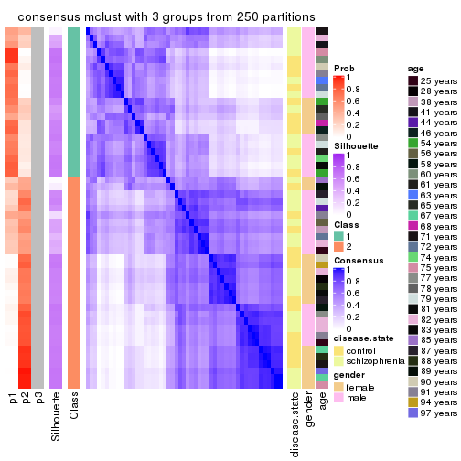
consensus_heatmap(res, k = 4)
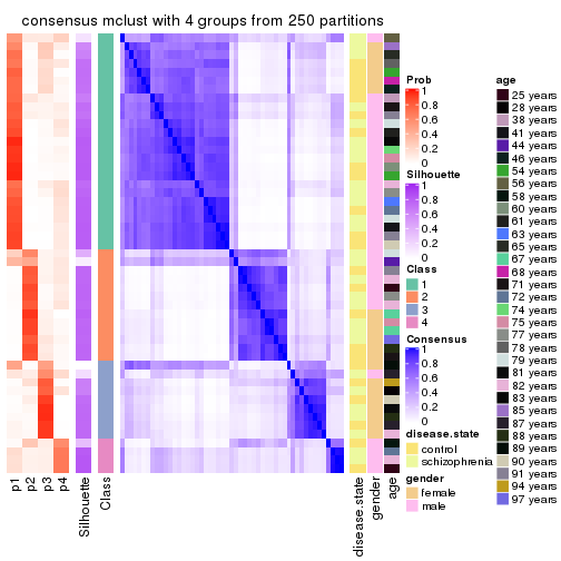
consensus_heatmap(res, k = 5)
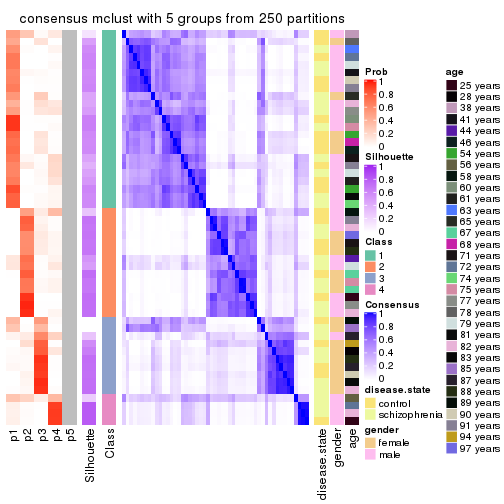
consensus_heatmap(res, k = 6)
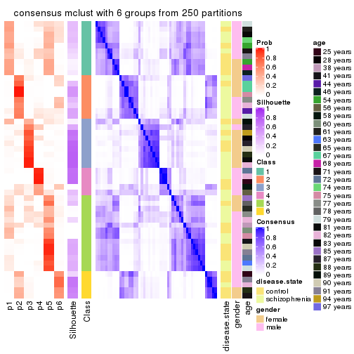
Heatmaps for the membership of samples in all partitions to see how consistent they are:
membership_heatmap(res, k = 2)
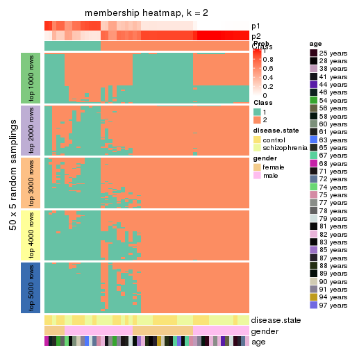
membership_heatmap(res, k = 3)
membership_heatmap(res, k = 4)
membership_heatmap(res, k = 5)
membership_heatmap(res, k = 6)
As soon as we have had the classes for columns, we can look for signatures which are significantly different between classes which can be candidate marks for certain classes. Following are the heatmaps for signatures.
Signature heatmaps where rows are scaled:
get_signatures(res, k = 2)
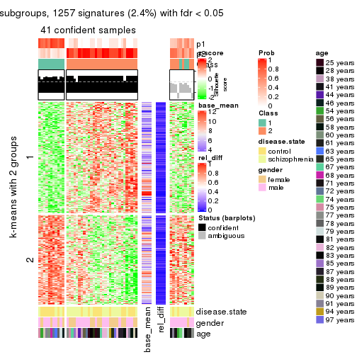
get_signatures(res, k = 3)
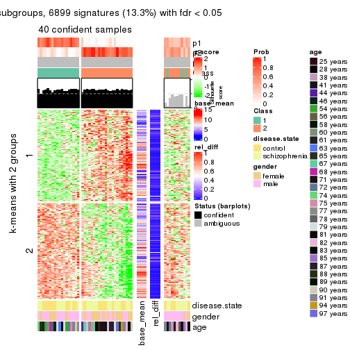
get_signatures(res, k = 4)
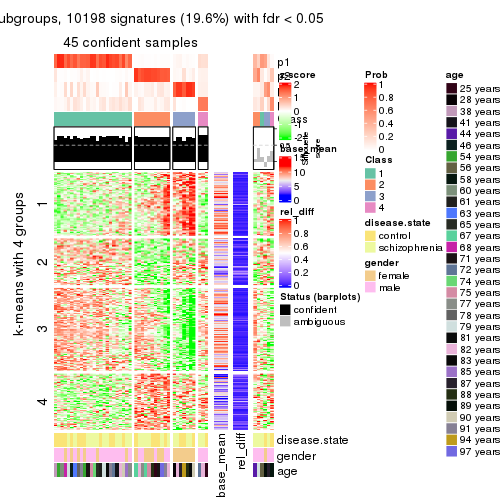
get_signatures(res, k = 5)
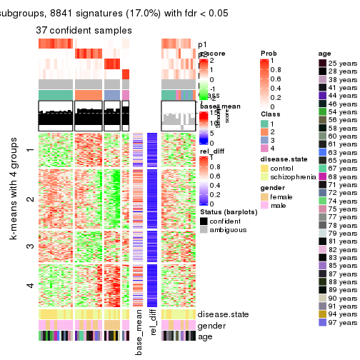
get_signatures(res, k = 6)
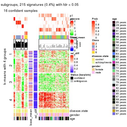
Signature heatmaps where rows are not scaled:
get_signatures(res, k = 2, scale_rows = FALSE)
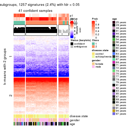
get_signatures(res, k = 3, scale_rows = FALSE)
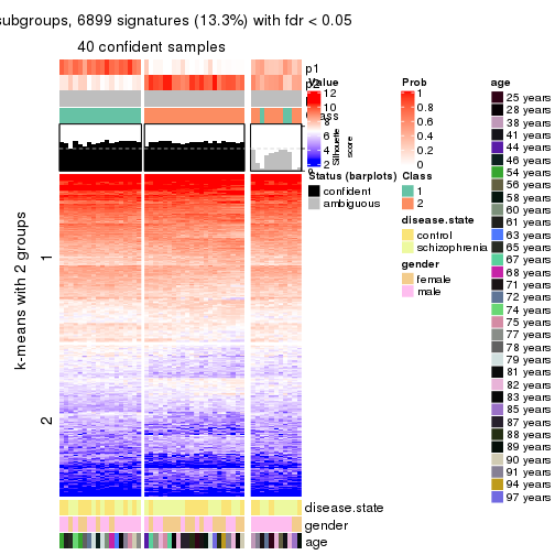
get_signatures(res, k = 4, scale_rows = FALSE)
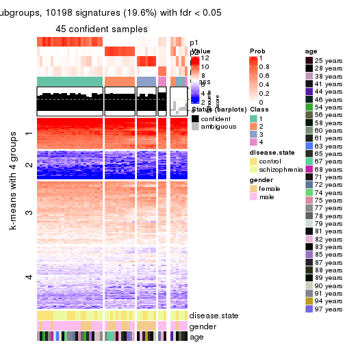
get_signatures(res, k = 5, scale_rows = FALSE)
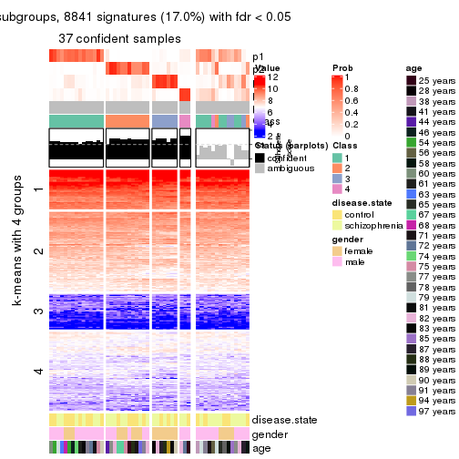
get_signatures(res, k = 6, scale_rows = FALSE)
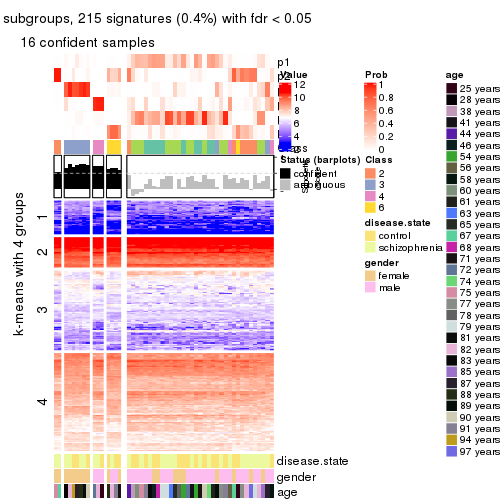
Compare the overlap of signatures from different k:
compare_signatures(res)
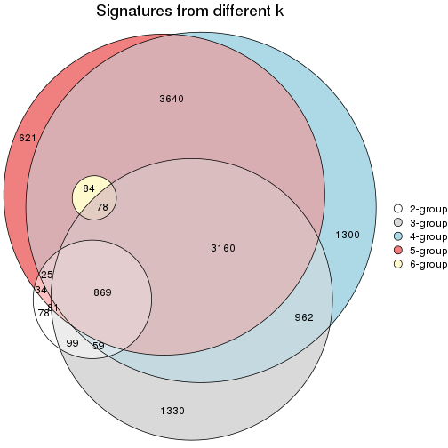
get_signature() returns a data frame invisibly. TO get the list of signatures, the function
call should be assigned to a variable explicitly. In following code, if plot argument is set
to FALSE, no heatmap is plotted while only the differential analysis is performed.
# code only for demonstration
tb = get_signature(res, k = ..., plot = FALSE)
An example of the output of tb is:
#>   which_row         fdr    mean_1    mean_2 scaled_mean_1 scaled_mean_2 km
#> 1        38 0.042760348  8.373488  9.131774    -0.5533452     0.5164555  1
#> 2        40 0.018707592  7.106213  8.469186    -0.6173731     0.5762149  1
#> 3        55 0.019134737 10.221463 11.207825    -0.6159697     0.5749050  1
#> 4        59 0.006059896  5.921854  7.869574    -0.6899429     0.6439467  1
#> 5        60 0.018055526  8.928898 10.211722    -0.6204761     0.5791110  1
#> 6        98 0.009384629 15.714769 14.887706     0.6635654    -0.6193277  2
...
The columns in tb are:
which_row: row indices corresponding to the input matrix.fdr: FDR for the differential test. mean_x: The mean value in group x.scaled_mean_x: The mean value in group x after rows are scaled.km: Row groups if k-means clustering is applied to rows.UMAP plot which shows how samples are separated.
dimension_reduction(res, k = 2, method = "UMAP")
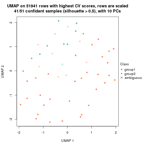
dimension_reduction(res, k = 3, method = "UMAP")
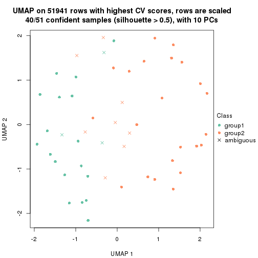
dimension_reduction(res, k = 4, method = "UMAP")
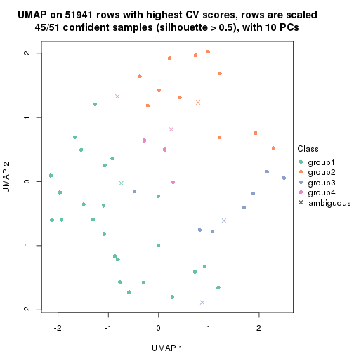
dimension_reduction(res, k = 5, method = "UMAP")
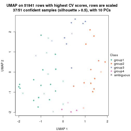
dimension_reduction(res, k = 6, method = "UMAP")
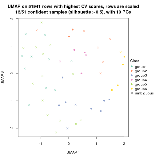
Following heatmap shows how subgroups are split when increasing k:
collect_classes(res)
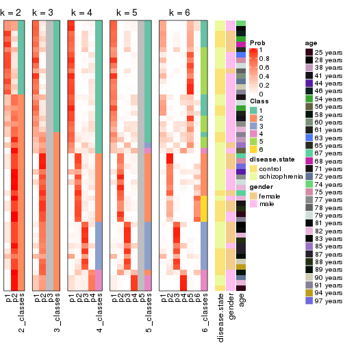
Test correlation between subgroups and known annotations. If the known annotation is numeric, one-way ANOVA test is applied, and if the known annotation is discrete, chi-squared contingency table test is applied.
test_to_known_factors(res)
#>            n disease.state(p) gender(p) age(p) k
#> CV:mclust 41            0.132   0.67274  0.397 2
#> CV:mclust 40            0.545   0.09671  0.350 3
#> CV:mclust 45            0.947   0.00152  0.841 4
#> CV:mclust 37            0.709   0.00182  0.762 5
#> CV:mclust 16            0.351   0.01000  0.418 6
If matrix rows can be associated to genes, consider to use functional_enrichment(res,
...) to perform function enrichment for the signature genes. See this vignette for more detailed explanations.
The object with results only for a single top-value method and a single partition method can be extracted as:
res = res_list["CV", "NMF"]
# you can also extract it by
# res = res_list["CV:NMF"]
A summary of res and all the functions that can be applied to it:
res
#> A 'ConsensusPartition' object with k = 2, 3, 4, 5, 6.
#>   On a matrix with 51941 rows and 51 columns.
#>   Top rows (1000, 2000, 3000, 4000, 5000) are extracted by 'CV' method.
#>   Subgroups are detected by 'NMF' method.
#>   Performed in total 1250 partitions by row resampling.
#>   Best k for subgroups seems to be 2.
#>
#> Following methods can be applied to this 'ConsensusPartition' object:
#>  [1] "cola_report"             "collect_classes"         "collect_plots"
#>  [4] "collect_stats"           "colnames"                "compare_signatures"
#>  [7] "consensus_heatmap"       "dimension_reduction"     "functional_enrichment"
#> [10] "get_anno_col"            "get_anno"                "get_classes"
#> [13] "get_consensus"           "get_matrix"              "get_membership"
#> [16] "get_param"               "get_signatures"          "get_stats"
#> [19] "is_best_k"               "is_stable_k"             "membership_heatmap"
#> [22] "ncol"                    "nrow"                    "plot_ecdf"
#> [25] "rownames"                "select_partition_number" "show"
#> [28] "suggest_best_k"          "test_to_known_factors"
collect_plots() function collects all the plots made from res for all k (number of partitions)
into one single page to provide an easy and fast comparison between different k.
collect_plots(res)
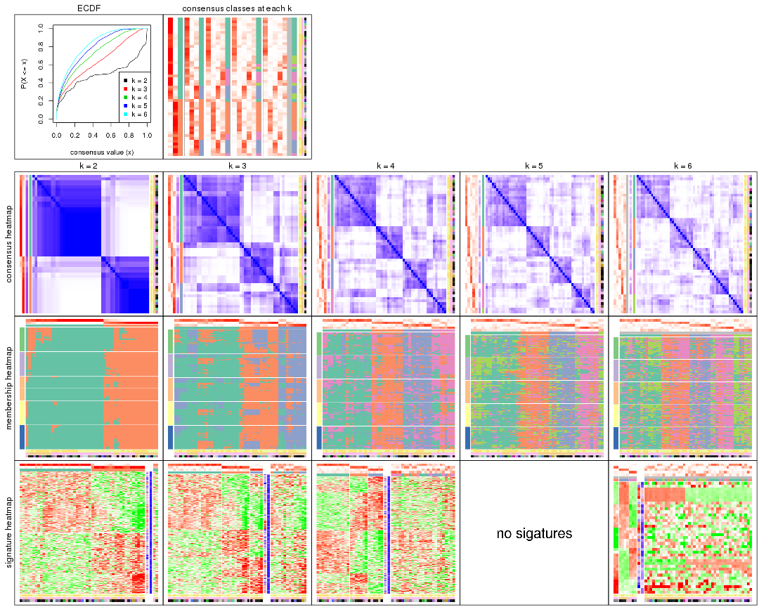
The plots are:
k and the heatmap of
predicted classes for each k.k.k.k.All the plots in panels can be made by individual functions and they are plotted later in this section.
select_partition_number() produces several plots showing different
statistics for choosing “optimized” k. There are following statistics:
k;k, the area increased is defined as \(A_k - A_{k-1}\).The detailed explanations of these statistics can be found in the cola vignette.
Generally speaking, lower PAC score, higher mean silhouette score or higher
concordance corresponds to better partition. Rand index and Jaccard index
measure how similar the current partition is compared to partition with k-1.
If they are too similar, we won't accept k is better than k-1.
select_partition_number(res)
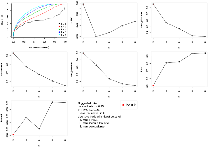
The numeric values for all these statistics can be obtained by get_stats().
get_stats(res)
#>   k 1-PAC mean_silhouette concordance area_increased  Rand Jaccard
#> 2 2 0.642           0.858       0.930         0.4939 0.506   0.506
#> 3 3 0.349           0.555       0.770         0.3261 0.808   0.637
#> 4 4 0.385           0.459       0.682         0.1365 0.821   0.551
#> 5 5 0.447           0.346       0.605         0.0679 0.931   0.757
#> 6 6 0.487           0.331       0.550         0.0425 0.937   0.753
suggest_best_k() suggests the best \(k\) based on these statistics. The rules are as follows:
suggest_best_k(res)
#> [1] 2
Following shows the table of the partitions (You need to click the show/hide
code output link to see it). The membership matrix (columns with name p*)
is inferred by
clue::cl_consensus()
function with the SE method. Basically the value in the membership matrix
represents the probability to belong to a certain group. The finall class
label for an item is determined with the group with highest probability it
belongs to.
In get_classes() function, the entropy is calculated from the membership
matrix and the silhouette score is calculated from the consensus matrix.
cbind(get_classes(res, k = 2), get_membership(res, k = 2))
#>           class entropy silhouette    p1    p2
#> GSM439800     2  0.6148      0.795 0.152 0.848
#> GSM439790     1  0.4815      0.872 0.896 0.104
#> GSM439827     2  0.0000      0.910 0.000 1.000
#> GSM439811     2  0.0000      0.910 0.000 1.000
#> GSM439795     2  0.0000      0.910 0.000 1.000
#> GSM439805     2  0.6973      0.747 0.188 0.812
#> GSM439781     1  0.7528      0.755 0.784 0.216
#> GSM439807     1  0.9522      0.475 0.628 0.372
#> GSM439820     2  0.0000      0.910 0.000 1.000
#> GSM439784     1  0.0000      0.928 1.000 0.000
#> GSM439824     2  0.9358      0.555 0.352 0.648
#> GSM439794     2  0.9209      0.596 0.336 0.664
#> GSM439809     1  0.0000      0.928 1.000 0.000
#> GSM439785     1  0.0376      0.926 0.996 0.004
#> GSM439803     1  0.0000      0.928 1.000 0.000
#> GSM439778     1  0.0000      0.928 1.000 0.000
#> GSM439791     1  0.0000      0.928 1.000 0.000
#> GSM439786     1  0.0000      0.928 1.000 0.000
#> GSM439828     2  0.1843      0.904 0.028 0.972
#> GSM439806     1  0.0000      0.928 1.000 0.000
#> GSM439815     1  0.0000      0.928 1.000 0.000
#> GSM439817     2  0.7219      0.784 0.200 0.800
#> GSM439796     1  0.9710      0.210 0.600 0.400
#> GSM439798     1  0.0000      0.928 1.000 0.000
#> GSM439821     2  0.0938      0.909 0.012 0.988
#> GSM439823     2  0.4690      0.866 0.100 0.900
#> GSM439813     1  0.0000      0.928 1.000 0.000
#> GSM439801     2  0.7376      0.776 0.208 0.792
#> GSM439810     1  0.4562      0.879 0.904 0.096
#> GSM439783     1  0.5629      0.846 0.868 0.132
#> GSM439826     2  0.0000      0.910 0.000 1.000
#> GSM439812     1  0.3584      0.897 0.932 0.068
#> GSM439818     2  0.0000      0.910 0.000 1.000
#> GSM439792     1  0.4298      0.884 0.912 0.088
#> GSM439802     1  0.7376      0.763 0.792 0.208
#> GSM439825     2  0.0000      0.910 0.000 1.000
#> GSM439780     1  0.2603      0.909 0.956 0.044
#> GSM439787     2  0.0000      0.910 0.000 1.000
#> GSM439808     2  0.0000      0.910 0.000 1.000
#> GSM439804     1  0.0672      0.924 0.992 0.008
#> GSM439822     2  0.0938      0.909 0.012 0.988
#> GSM439816     1  0.3274      0.889 0.940 0.060
#> GSM439789     1  0.0000      0.928 1.000 0.000
#> GSM439799     2  0.3879      0.881 0.076 0.924
#> GSM439814     1  0.0000      0.928 1.000 0.000
#> GSM439782     1  0.0000      0.928 1.000 0.000
#> GSM439779     1  0.0000      0.928 1.000 0.000
#> GSM439793     1  0.0000      0.928 1.000 0.000
#> GSM439788     1  0.0000      0.928 1.000 0.000
#> GSM439797     1  0.4298      0.861 0.912 0.088
#> GSM439819     2  0.0938      0.909 0.012 0.988
cbind(get_classes(res, k = 3), get_membership(res, k = 3))
#>           class entropy silhouette    p1    p2    p3
#> GSM439800     3   0.296     0.6235 0.008 0.080 0.912
#> GSM439790     3   0.625     0.1840 0.376 0.004 0.620
#> GSM439827     2   0.546     0.6244 0.020 0.776 0.204
#> GSM439811     2   0.584     0.6248 0.036 0.768 0.196
#> GSM439795     3   0.334     0.5795 0.000 0.120 0.880
#> GSM439805     3   0.203     0.6486 0.016 0.032 0.952
#> GSM439781     3   0.570     0.4820 0.252 0.012 0.736
#> GSM439807     3   0.249     0.6552 0.048 0.016 0.936
#> GSM439820     2   0.627     0.3280 0.000 0.548 0.452
#> GSM439784     1   0.245     0.7431 0.936 0.052 0.012
#> GSM439824     2   0.615     0.0852 0.408 0.592 0.000
#> GSM439794     2   0.695     0.2570 0.352 0.620 0.028
#> GSM439809     1   0.447     0.7347 0.852 0.028 0.120
#> GSM439785     1   0.536     0.6137 0.724 0.276 0.000
#> GSM439803     1   0.603     0.6779 0.752 0.212 0.036
#> GSM439778     1   0.447     0.6957 0.820 0.004 0.176
#> GSM439791     1   0.175     0.7457 0.952 0.000 0.048
#> GSM439786     1   0.843     0.4417 0.552 0.100 0.348
#> GSM439828     2   0.134     0.6837 0.012 0.972 0.016
#> GSM439806     1   0.336     0.7506 0.908 0.056 0.036
#> GSM439815     1   0.517     0.7335 0.824 0.048 0.128
#> GSM439817     2   0.355     0.6113 0.132 0.868 0.000
#> GSM439796     1   0.776     0.1819 0.488 0.464 0.048
#> GSM439798     1   0.857     0.2569 0.476 0.096 0.428
#> GSM439821     2   0.473     0.6392 0.004 0.800 0.196
#> GSM439823     2   0.205     0.6763 0.028 0.952 0.020
#> GSM439813     1   0.455     0.6758 0.800 0.000 0.200
#> GSM439801     3   0.776    -0.1514 0.048 0.464 0.488
#> GSM439810     1   0.517     0.6373 0.784 0.012 0.204
#> GSM439783     1   0.572     0.5515 0.704 0.004 0.292
#> GSM439826     2   0.567     0.6441 0.060 0.800 0.140
#> GSM439812     1   0.435     0.6760 0.828 0.004 0.168
#> GSM439818     2   0.615     0.4147 0.000 0.592 0.408
#> GSM439792     1   0.596     0.5874 0.720 0.016 0.264
#> GSM439802     3   0.327     0.6446 0.104 0.004 0.892
#> GSM439825     2   0.568     0.5438 0.000 0.684 0.316
#> GSM439780     3   0.598     0.3465 0.328 0.004 0.668
#> GSM439787     3   0.470     0.4611 0.000 0.212 0.788
#> GSM439808     3   0.593     0.1266 0.000 0.356 0.644
#> GSM439804     1   0.663     0.6141 0.692 0.272 0.036
#> GSM439822     2   0.188     0.6870 0.004 0.952 0.044
#> GSM439816     1   0.598     0.5189 0.668 0.328 0.004
#> GSM439789     1   0.153     0.7440 0.960 0.040 0.000
#> GSM439799     2   0.546     0.6252 0.016 0.768 0.216
#> GSM439814     1   0.230     0.7372 0.936 0.060 0.004
#> GSM439782     1   0.592     0.6100 0.724 0.016 0.260
#> GSM439779     1   0.153     0.7454 0.960 0.000 0.040
#> GSM439793     1   0.337     0.7493 0.904 0.024 0.072
#> GSM439788     1   0.487     0.7202 0.824 0.024 0.152
#> GSM439797     1   0.599     0.4785 0.632 0.368 0.000
#> GSM439819     2   0.429     0.6628 0.004 0.832 0.164
cbind(get_classes(res, k = 4), get_membership(res, k = 4))
#>           class entropy silhouette    p1    p2    p3    p4
#> GSM439800     3   0.646    0.56157 0.012 0.124 0.672 0.192
#> GSM439790     3   0.673    0.42009 0.228 0.008 0.632 0.132
#> GSM439827     2   0.718    0.45220 0.208 0.644 0.076 0.072
#> GSM439811     2   0.738    0.44643 0.196 0.636 0.092 0.076
#> GSM439795     3   0.385    0.63974 0.000 0.116 0.840 0.044
#> GSM439805     3   0.345    0.66347 0.008 0.092 0.872 0.028
#> GSM439781     3   0.788    0.49943 0.164 0.188 0.588 0.060
#> GSM439807     3   0.333    0.66575 0.016 0.056 0.888 0.040
#> GSM439820     2   0.506    0.46481 0.008 0.728 0.240 0.024
#> GSM439784     1   0.563    0.56531 0.772 0.096 0.052 0.080
#> GSM439824     1   0.747    0.13056 0.496 0.332 0.004 0.168
#> GSM439794     4   0.614    0.33658 0.096 0.252 0.000 0.652
#> GSM439809     1   0.403    0.64847 0.836 0.000 0.072 0.092
#> GSM439785     1   0.575    0.21382 0.528 0.020 0.004 0.448
#> GSM439803     4   0.446    0.48703 0.176 0.024 0.008 0.792
#> GSM439778     1   0.663    0.44520 0.600 0.004 0.100 0.296
#> GSM439791     1   0.404    0.62406 0.804 0.000 0.020 0.176
#> GSM439786     4   0.743    0.16348 0.288 0.000 0.208 0.504
#> GSM439828     2   0.440    0.65373 0.048 0.800 0.000 0.152
#> GSM439806     1   0.272    0.65517 0.908 0.012 0.012 0.068
#> GSM439815     4   0.712    0.01414 0.384 0.004 0.116 0.496
#> GSM439817     2   0.695    0.46610 0.148 0.592 0.004 0.256
#> GSM439796     4   0.459    0.48642 0.068 0.136 0.000 0.796
#> GSM439798     3   0.856   -0.09042 0.236 0.032 0.380 0.352
#> GSM439821     2   0.511    0.62496 0.000 0.744 0.060 0.196
#> GSM439823     2   0.539    0.25809 0.012 0.528 0.000 0.460
#> GSM439813     1   0.716    0.37421 0.552 0.004 0.148 0.296
#> GSM439801     4   0.835   -0.00478 0.016 0.296 0.308 0.380
#> GSM439810     1   0.623    0.56181 0.700 0.024 0.192 0.084
#> GSM439783     1   0.672    0.37258 0.596 0.040 0.324 0.040
#> GSM439826     2   0.545    0.64166 0.048 0.752 0.024 0.176
#> GSM439812     1   0.534    0.63990 0.784 0.032 0.088 0.096
#> GSM439818     2   0.535    0.60745 0.000 0.736 0.180 0.084
#> GSM439792     1   0.639    0.54372 0.704 0.060 0.180 0.056
#> GSM439802     3   0.404    0.58921 0.020 0.000 0.804 0.176
#> GSM439825     2   0.479    0.65966 0.000 0.788 0.104 0.108
#> GSM439780     3   0.600    0.48475 0.120 0.004 0.700 0.176
#> GSM439787     3   0.572    0.51902 0.012 0.264 0.684 0.040
#> GSM439808     3   0.595    0.33216 0.004 0.380 0.580 0.036
#> GSM439804     4   0.430    0.53514 0.108 0.056 0.008 0.828
#> GSM439822     2   0.430    0.61748 0.000 0.752 0.008 0.240
#> GSM439816     1   0.560    0.52825 0.736 0.144 0.004 0.116
#> GSM439789     1   0.463    0.56864 0.740 0.004 0.012 0.244
#> GSM439799     4   0.577   -0.12632 0.000 0.404 0.032 0.564
#> GSM439814     1   0.263    0.64738 0.912 0.016 0.008 0.064
#> GSM439782     4   0.732    0.03343 0.352 0.004 0.144 0.500
#> GSM439779     1   0.340    0.65610 0.876 0.004 0.044 0.076
#> GSM439793     1   0.555    0.61399 0.772 0.040 0.076 0.112
#> GSM439788     1   0.618    0.58409 0.696 0.008 0.144 0.152
#> GSM439797     1   0.690    0.25250 0.516 0.096 0.004 0.384
#> GSM439819     2   0.313    0.67843 0.004 0.884 0.024 0.088
cbind(get_classes(res, k = 5), get_membership(res, k = 5))
#>           class entropy silhouette    p1    p2    p3    p4    p5
#> GSM439800     3   0.758    0.48340 0.052 0.100 0.592 0.124 0.132
#> GSM439790     3   0.723    0.02408 0.216 0.000 0.508 0.052 0.224
#> GSM439827     2   0.660    0.45679 0.100 0.596 0.044 0.008 0.252
#> GSM439811     2   0.669    0.45035 0.092 0.592 0.056 0.008 0.252
#> GSM439795     3   0.424    0.58059 0.004 0.104 0.812 0.048 0.032
#> GSM439805     3   0.398    0.58654 0.000 0.096 0.816 0.012 0.076
#> GSM439781     3   0.778    0.19385 0.120 0.128 0.388 0.000 0.364
#> GSM439807     3   0.406    0.58678 0.020 0.040 0.804 0.000 0.136
#> GSM439820     2   0.599    0.41668 0.004 0.632 0.192 0.008 0.164
#> GSM439784     1   0.623    0.28008 0.592 0.104 0.020 0.004 0.280
#> GSM439824     1   0.771   -0.00853 0.408 0.352 0.000 0.112 0.128
#> GSM439794     4   0.585    0.46088 0.056 0.192 0.024 0.692 0.036
#> GSM439809     1   0.381    0.47074 0.840 0.004 0.052 0.024 0.080
#> GSM439785     4   0.708   -0.22417 0.348 0.040 0.000 0.460 0.152
#> GSM439803     4   0.399    0.41132 0.116 0.016 0.016 0.824 0.028
#> GSM439778     1   0.686    0.14889 0.580 0.000 0.064 0.200 0.156
#> GSM439791     1   0.476    0.40831 0.764 0.004 0.012 0.104 0.116
#> GSM439786     5   0.820    0.56774 0.248 0.000 0.112 0.300 0.340
#> GSM439828     2   0.450    0.56588 0.036 0.792 0.000 0.100 0.072
#> GSM439806     1   0.506    0.40716 0.724 0.028 0.012 0.028 0.208
#> GSM439815     1   0.827    0.12227 0.408 0.008 0.148 0.284 0.152
#> GSM439817     2   0.735    0.32715 0.084 0.524 0.000 0.216 0.176
#> GSM439796     4   0.223    0.50254 0.020 0.036 0.004 0.924 0.016
#> GSM439798     5   0.853    0.58607 0.204 0.028 0.180 0.144 0.444
#> GSM439821     2   0.606    0.48001 0.000 0.656 0.048 0.192 0.104
#> GSM439823     4   0.566    0.16803 0.004 0.344 0.000 0.572 0.080
#> GSM439813     1   0.697    0.32600 0.592 0.000 0.132 0.156 0.120
#> GSM439801     4   0.807    0.17109 0.000 0.232 0.212 0.424 0.132
#> GSM439810     1   0.695    0.38613 0.588 0.024 0.180 0.028 0.180
#> GSM439783     1   0.771    0.26038 0.512 0.044 0.264 0.044 0.136
#> GSM439826     2   0.724    0.46910 0.044 0.572 0.032 0.224 0.128
#> GSM439812     1   0.629    0.46091 0.664 0.032 0.068 0.040 0.196
#> GSM439818     2   0.723    0.38731 0.000 0.532 0.232 0.076 0.160
#> GSM439792     1   0.605    0.38375 0.664 0.032 0.156 0.004 0.144
#> GSM439802     3   0.428    0.50979 0.036 0.000 0.808 0.084 0.072
#> GSM439825     2   0.591    0.54878 0.000 0.688 0.136 0.108 0.068
#> GSM439780     3   0.656    0.35805 0.152 0.000 0.616 0.060 0.172
#> GSM439787     3   0.675    0.38144 0.012 0.260 0.500 0.000 0.228
#> GSM439808     3   0.625    0.38553 0.004 0.252 0.560 0.000 0.184
#> GSM439804     4   0.360    0.47782 0.052 0.024 0.024 0.864 0.036
#> GSM439822     2   0.561    0.43931 0.004 0.636 0.016 0.284 0.060
#> GSM439816     1   0.712    0.35079 0.564 0.204 0.004 0.068 0.160
#> GSM439789     1   0.418    0.45866 0.788 0.012 0.000 0.152 0.048
#> GSM439799     4   0.546    0.38370 0.004 0.224 0.052 0.688 0.032
#> GSM439814     1   0.499    0.48782 0.756 0.044 0.004 0.052 0.144
#> GSM439782     4   0.785   -0.39074 0.348 0.000 0.084 0.372 0.196
#> GSM439779     1   0.360    0.45520 0.844 0.004 0.020 0.028 0.104
#> GSM439793     1   0.612    0.13332 0.576 0.044 0.032 0.012 0.336
#> GSM439788     1   0.599    0.17579 0.600 0.004 0.076 0.020 0.300
#> GSM439797     1   0.798   -0.34004 0.320 0.076 0.000 0.304 0.300
#> GSM439819     2   0.496    0.55017 0.000 0.744 0.020 0.140 0.096
cbind(get_classes(res, k = 6), get_membership(res, k = 6))
#>           class entropy silhouette    p1    p2    p3    p4    p5 p6
#> GSM439800     3   0.735     0.4479 0.096 0.052 0.468 0.040 0.024 NA
#> GSM439790     5   0.796     0.0726 0.080 0.000 0.304 0.080 0.376 NA
#> GSM439827     2   0.742     0.3990 0.088 0.516 0.072 0.000 0.192 NA
#> GSM439811     2   0.791     0.3566 0.096 0.440 0.076 0.000 0.188 NA
#> GSM439795     3   0.381     0.5763 0.000 0.028 0.828 0.044 0.028 NA
#> GSM439805     3   0.528     0.5174 0.000 0.040 0.708 0.020 0.140 NA
#> GSM439781     5   0.718     0.0881 0.040 0.076 0.220 0.000 0.512 NA
#> GSM439807     3   0.554     0.5591 0.040 0.012 0.668 0.008 0.064 NA
#> GSM439820     2   0.702     0.3028 0.032 0.504 0.200 0.012 0.024 NA
#> GSM439784     1   0.555     0.1333 0.468 0.072 0.004 0.000 0.440 NA
#> GSM439824     1   0.723     0.1511 0.484 0.288 0.000 0.080 0.064 NA
#> GSM439794     4   0.670     0.4730 0.112 0.120 0.028 0.632 0.040 NA
#> GSM439809     1   0.547     0.3885 0.668 0.000 0.056 0.028 0.212 NA
#> GSM439785     4   0.709     0.0639 0.184 0.048 0.000 0.500 0.228 NA
#> GSM439803     4   0.411     0.5040 0.096 0.008 0.004 0.804 0.048 NA
#> GSM439778     1   0.806    -0.0620 0.324 0.000 0.052 0.188 0.324 NA
#> GSM439791     1   0.601     0.3101 0.588 0.004 0.008 0.088 0.268 NA
#> GSM439786     5   0.668     0.2550 0.064 0.016 0.048 0.308 0.532 NA
#> GSM439828     2   0.425     0.5370 0.028 0.800 0.000 0.084 0.044 NA
#> GSM439806     1   0.548     0.2818 0.572 0.028 0.000 0.016 0.344 NA
#> GSM439815     1   0.798     0.2592 0.436 0.008 0.116 0.164 0.048 NA
#> GSM439817     2   0.750     0.3279 0.056 0.500 0.000 0.180 0.164 NA
#> GSM439796     4   0.362     0.5447 0.032 0.064 0.004 0.844 0.020 NA
#> GSM439798     5   0.600     0.4243 0.052 0.032 0.088 0.124 0.684 NA
#> GSM439821     2   0.577     0.4680 0.000 0.684 0.076 0.136 0.048 NA
#> GSM439823     4   0.567     0.0553 0.000 0.376 0.000 0.520 0.052 NA
#> GSM439813     1   0.671     0.3781 0.592 0.000 0.096 0.100 0.044 NA
#> GSM439801     4   0.810     0.1325 0.000 0.172 0.256 0.384 0.128 NA
#> GSM439810     1   0.705     0.3357 0.544 0.020 0.156 0.008 0.088 NA
#> GSM439783     1   0.830     0.1715 0.380 0.020 0.164 0.036 0.140 NA
#> GSM439826     2   0.687     0.4604 0.060 0.512 0.012 0.168 0.004 NA
#> GSM439812     1   0.561     0.4407 0.680 0.020 0.072 0.012 0.032 NA
#> GSM439818     2   0.687     0.3351 0.000 0.416 0.204 0.052 0.004 NA
#> GSM439792     1   0.697     0.2499 0.512 0.032 0.136 0.000 0.256 NA
#> GSM439802     3   0.524     0.5327 0.012 0.000 0.716 0.072 0.080 NA
#> GSM439825     2   0.669     0.4359 0.000 0.560 0.144 0.060 0.028 NA
#> GSM439780     3   0.761     0.3016 0.076 0.000 0.448 0.052 0.188 NA
#> GSM439787     3   0.670     0.3450 0.004 0.196 0.540 0.004 0.180 NA
#> GSM439808     3   0.703     0.3619 0.012 0.188 0.484 0.008 0.052 NA
#> GSM439804     4   0.343     0.5385 0.052 0.012 0.008 0.856 0.024 NA
#> GSM439822     2   0.563     0.4216 0.016 0.636 0.016 0.240 0.008 NA
#> GSM439816     1   0.660     0.3906 0.608 0.100 0.004 0.048 0.064 NA
#> GSM439789     1   0.461     0.4463 0.752 0.000 0.000 0.100 0.092 NA
#> GSM439799     4   0.453     0.4201 0.000 0.196 0.012 0.732 0.028 NA
#> GSM439814     1   0.311     0.4838 0.868 0.020 0.004 0.016 0.020 NA
#> GSM439782     4   0.825    -0.1541 0.184 0.000 0.060 0.364 0.236 NA
#> GSM439779     1   0.439     0.3997 0.724 0.000 0.012 0.028 0.220 NA
#> GSM439793     5   0.553     0.1626 0.300 0.044 0.004 0.024 0.608 NA
#> GSM439788     5   0.612     0.1319 0.328 0.012 0.044 0.048 0.552 NA
#> GSM439797     5   0.709     0.2141 0.124 0.104 0.000 0.280 0.476 NA
#> GSM439819     2   0.503     0.5087 0.000 0.744 0.044 0.112 0.056 NA
Heatmaps for the consensus matrix. It visualizes the probability of two samples to be in a same group.
consensus_heatmap(res, k = 2)
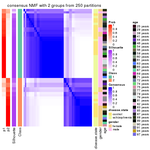
consensus_heatmap(res, k = 3)
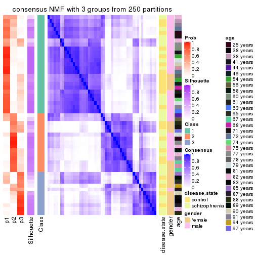
consensus_heatmap(res, k = 4)
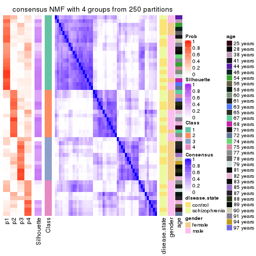
consensus_heatmap(res, k = 5)
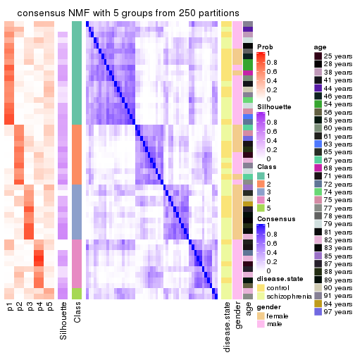
consensus_heatmap(res, k = 6)
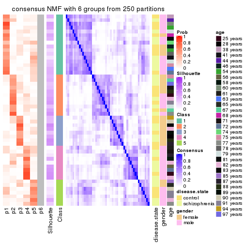
Heatmaps for the membership of samples in all partitions to see how consistent they are:
membership_heatmap(res, k = 2)
membership_heatmap(res, k = 3)
membership_heatmap(res, k = 4)
membership_heatmap(res, k = 5)
membership_heatmap(res, k = 6)
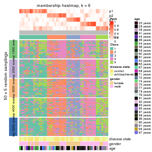
As soon as we have had the classes for columns, we can look for signatures which are significantly different between classes which can be candidate marks for certain classes. Following are the heatmaps for signatures.
Signature heatmaps where rows are scaled:
get_signatures(res, k = 2)

get_signatures(res, k = 3)
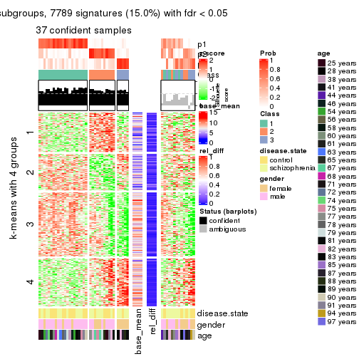
get_signatures(res, k = 4)
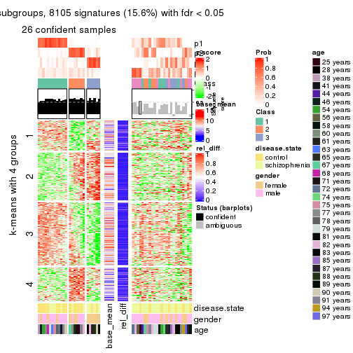
get_signatures(res, k = 5)

get_signatures(res, k = 6)
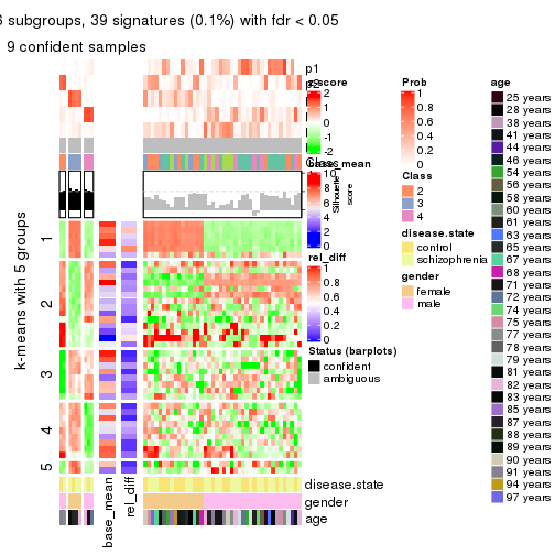
Signature heatmaps where rows are not scaled:
get_signatures(res, k = 2, scale_rows = FALSE)
get_signatures(res, k = 3, scale_rows = FALSE)
get_signatures(res, k = 4, scale_rows = FALSE)
get_signatures(res, k = 5, scale_rows = FALSE)

get_signatures(res, k = 6, scale_rows = FALSE)
Compare the overlap of signatures from different k:
compare_signatures(res)
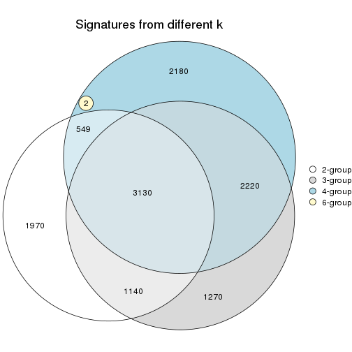
get_signature() returns a data frame invisibly. TO get the list of signatures, the function
call should be assigned to a variable explicitly. In following code, if plot argument is set
to FALSE, no heatmap is plotted while only the differential analysis is performed.
# code only for demonstration
tb = get_signature(res, k = ..., plot = FALSE)
An example of the output of tb is:
#>   which_row         fdr    mean_1    mean_2 scaled_mean_1 scaled_mean_2 km
#> 1        38 0.042760348  8.373488  9.131774    -0.5533452     0.5164555  1
#> 2        40 0.018707592  7.106213  8.469186    -0.6173731     0.5762149  1
#> 3        55 0.019134737 10.221463 11.207825    -0.6159697     0.5749050  1
#> 4        59 0.006059896  5.921854  7.869574    -0.6899429     0.6439467  1
#> 5        60 0.018055526  8.928898 10.211722    -0.6204761     0.5791110  1
#> 6        98 0.009384629 15.714769 14.887706     0.6635654    -0.6193277  2
...
The columns in tb are:
which_row: row indices corresponding to the input matrix.fdr: FDR for the differential test. mean_x: The mean value in group x.scaled_mean_x: The mean value in group x after rows are scaled.km: Row groups if k-means clustering is applied to rows.UMAP plot which shows how samples are separated.
dimension_reduction(res, k = 2, method = "UMAP")
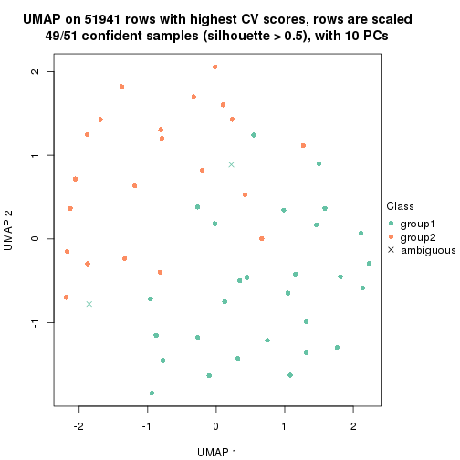
dimension_reduction(res, k = 3, method = "UMAP")
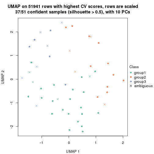
dimension_reduction(res, k = 4, method = "UMAP")
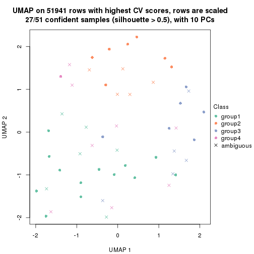
dimension_reduction(res, k = 5, method = "UMAP")
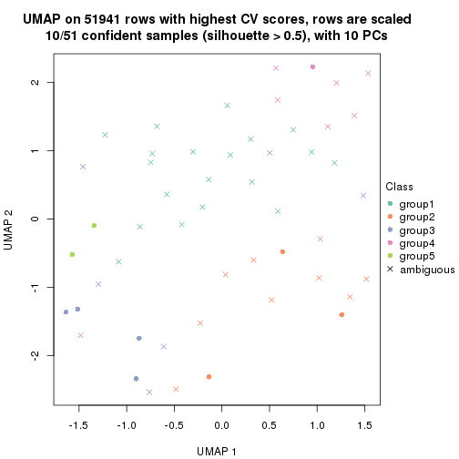
dimension_reduction(res, k = 6, method = "UMAP")
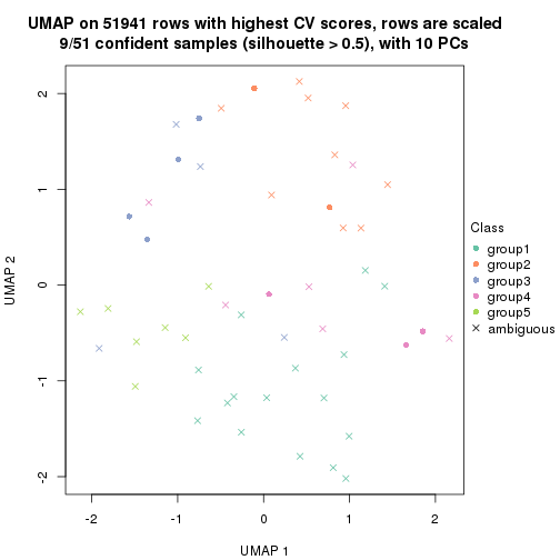
Following heatmap shows how subgroups are split when increasing k:
collect_classes(res)
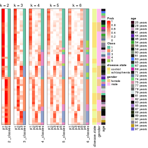
Test correlation between subgroups and known annotations. If the known annotation is numeric, one-way ANOVA test is applied, and if the known annotation is discrete, chi-squared contingency table test is applied.
test_to_known_factors(res)
#>         n disease.state(p) gender(p) age(p) k
#> CV:NMF 49            0.432   0.16255  0.657 2
#> CV:NMF 37            0.318   0.00299  0.460 3
#> CV:NMF 27            0.350   0.01340  0.862 4
#> CV:NMF 10            0.354   0.06200  0.735 5
#> CV:NMF  9            0.829   0.01111  0.353 6
If matrix rows can be associated to genes, consider to use functional_enrichment(res,
...) to perform function enrichment for the signature genes. See this vignette for more detailed explanations.
The object with results only for a single top-value method and a single partition method can be extracted as:
res = res_list["MAD", "hclust"]
# you can also extract it by
# res = res_list["MAD:hclust"]
A summary of res and all the functions that can be applied to it:
res
#> A 'ConsensusPartition' object with k = 2, 3, 4, 5, 6.
#>   On a matrix with 51941 rows and 51 columns.
#>   Top rows (1000, 2000, 3000, 4000, 5000) are extracted by 'MAD' method.
#>   Subgroups are detected by 'hclust' method.
#>   Performed in total 1250 partitions by row resampling.
#>   Best k for subgroups seems to be 2.
#>
#> Following methods can be applied to this 'ConsensusPartition' object:
#>  [1] "cola_report"             "collect_classes"         "collect_plots"
#>  [4] "collect_stats"           "colnames"                "compare_signatures"
#>  [7] "consensus_heatmap"       "dimension_reduction"     "functional_enrichment"
#> [10] "get_anno_col"            "get_anno"                "get_classes"
#> [13] "get_consensus"           "get_matrix"              "get_membership"
#> [16] "get_param"               "get_signatures"          "get_stats"
#> [19] "is_best_k"               "is_stable_k"             "membership_heatmap"
#> [22] "ncol"                    "nrow"                    "plot_ecdf"
#> [25] "rownames"                "select_partition_number" "show"
#> [28] "suggest_best_k"          "test_to_known_factors"
collect_plots() function collects all the plots made from res for all k (number of partitions)
into one single page to provide an easy and fast comparison between different k.
collect_plots(res)
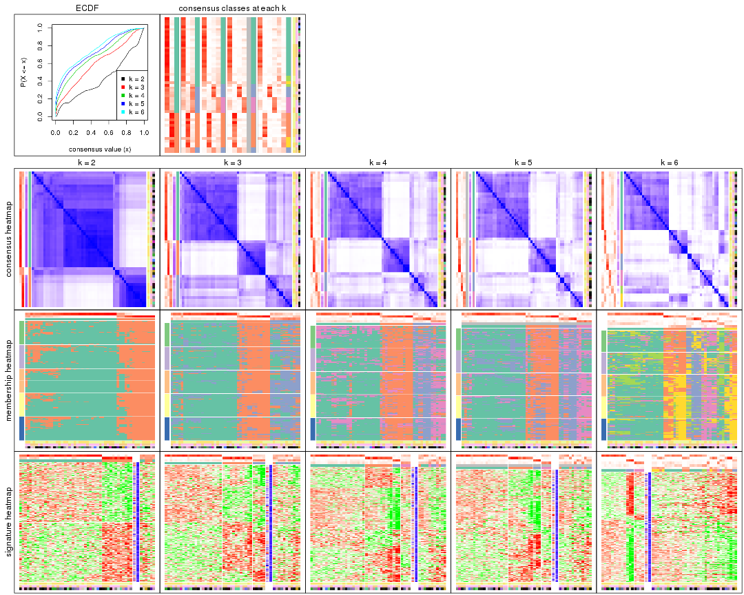
The plots are:
k and the heatmap of
predicted classes for each k.k.k.k.All the plots in panels can be made by individual functions and they are plotted later in this section.
select_partition_number() produces several plots showing different
statistics for choosing “optimized” k. There are following statistics:
k;k, the area increased is defined as \(A_k - A_{k-1}\).The detailed explanations of these statistics can be found in the cola vignette.
Generally speaking, lower PAC score, higher mean silhouette score or higher
concordance corresponds to better partition. Rand index and Jaccard index
measure how similar the current partition is compared to partition with k-1.
If they are too similar, we won't accept k is better than k-1.
select_partition_number(res)
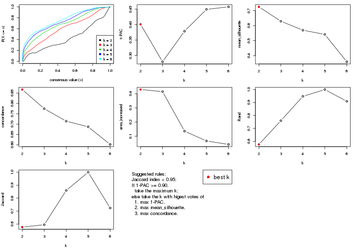
The numeric values for all these statistics can be obtained by get_stats().
get_stats(res)
#>   k 1-PAC mean_silhouette concordance area_increased  Rand Jaccard
#> 2 2 0.401           0.725       0.867         0.4291 0.576   0.576
#> 3 3 0.279           0.629       0.775         0.4143 0.760   0.595
#> 4 4 0.379           0.570       0.714         0.1359 0.947   0.859
#> 5 5 0.449           0.541       0.687         0.0667 1.000   1.000
#> 6 6 0.457           0.359       0.602         0.0422 0.909   0.724
suggest_best_k() suggests the best \(k\) based on these statistics. The rules are as follows:
suggest_best_k(res)
#> [1] 2
Following shows the table of the partitions (You need to click the show/hide
code output link to see it). The membership matrix (columns with name p*)
is inferred by
clue::cl_consensus()
function with the SE method. Basically the value in the membership matrix
represents the probability to belong to a certain group. The finall class
label for an item is determined with the group with highest probability it
belongs to.
In get_classes() function, the entropy is calculated from the membership
matrix and the silhouette score is calculated from the consensus matrix.
cbind(get_classes(res, k = 2), get_membership(res, k = 2))
#>           class entropy silhouette    p1    p2
#> GSM439800     1  0.8016     0.7304 0.756 0.244
#> GSM439790     1  0.1633     0.8581 0.976 0.024
#> GSM439827     2  0.0938     0.8210 0.012 0.988
#> GSM439811     2  0.1414     0.8214 0.020 0.980
#> GSM439795     1  0.9000     0.5972 0.684 0.316
#> GSM439805     1  0.7745     0.7401 0.772 0.228
#> GSM439781     1  0.3733     0.8544 0.928 0.072
#> GSM439807     2  1.0000    -0.1104 0.500 0.500
#> GSM439820     2  0.7299     0.6764 0.204 0.796
#> GSM439784     1  0.4690     0.8462 0.900 0.100
#> GSM439824     2  0.9963     0.0542 0.464 0.536
#> GSM439794     1  0.8386     0.6912 0.732 0.268
#> GSM439809     1  0.1184     0.8578 0.984 0.016
#> GSM439785     1  0.6623     0.8001 0.828 0.172
#> GSM439803     1  0.7453     0.7662 0.788 0.212
#> GSM439778     1  0.1633     0.8581 0.976 0.024
#> GSM439791     1  0.2778     0.8591 0.952 0.048
#> GSM439786     1  0.1414     0.8537 0.980 0.020
#> GSM439828     2  0.0938     0.8210 0.012 0.988
#> GSM439806     1  0.1184     0.8554 0.984 0.016
#> GSM439815     1  0.2778     0.8534 0.952 0.048
#> GSM439817     2  0.6148     0.7481 0.152 0.848
#> GSM439796     1  0.8499     0.6813 0.724 0.276
#> GSM439798     1  0.2236     0.8581 0.964 0.036
#> GSM439821     2  0.0672     0.8181 0.008 0.992
#> GSM439823     2  0.6438     0.7255 0.164 0.836
#> GSM439813     1  0.0672     0.8516 0.992 0.008
#> GSM439801     1  0.9087     0.5931 0.676 0.324
#> GSM439810     1  0.0376     0.8516 0.996 0.004
#> GSM439783     1  0.5842     0.8182 0.860 0.140
#> GSM439826     2  0.1633     0.8182 0.024 0.976
#> GSM439812     1  0.0938     0.8535 0.988 0.012
#> GSM439818     2  0.1414     0.8180 0.020 0.980
#> GSM439792     1  0.2423     0.8592 0.960 0.040
#> GSM439802     1  0.2778     0.8552 0.952 0.048
#> GSM439825     2  0.1184     0.8201 0.016 0.984
#> GSM439780     1  0.0938     0.8541 0.988 0.012
#> GSM439787     1  0.9580     0.4514 0.620 0.380
#> GSM439808     2  0.9998    -0.0835 0.492 0.508
#> GSM439804     1  0.8443     0.6859 0.728 0.272
#> GSM439822     2  0.2948     0.8137 0.052 0.948
#> GSM439816     1  0.9833     0.2780 0.576 0.424
#> GSM439789     1  0.1633     0.8581 0.976 0.024
#> GSM439799     1  0.9993     0.1556 0.516 0.484
#> GSM439814     1  0.1184     0.8555 0.984 0.016
#> GSM439782     1  0.0376     0.8512 0.996 0.004
#> GSM439779     1  0.1633     0.8586 0.976 0.024
#> GSM439793     1  0.3431     0.8556 0.936 0.064
#> GSM439788     1  0.3114     0.8574 0.944 0.056
#> GSM439797     1  0.6801     0.7912 0.820 0.180
#> GSM439819     2  0.0672     0.8181 0.008 0.992
cbind(get_classes(res, k = 3), get_membership(res, k = 3))
#>           class entropy silhouette    p1    p2    p3
#> GSM439800     3  0.8233     0.5708 0.272 0.116 0.612
#> GSM439790     1  0.3769     0.7902 0.880 0.016 0.104
#> GSM439827     2  0.0592     0.8104 0.000 0.988 0.012
#> GSM439811     2  0.0983     0.8106 0.004 0.980 0.016
#> GSM439795     3  0.7199     0.5989 0.204 0.092 0.704
#> GSM439805     3  0.8257     0.4027 0.372 0.084 0.544
#> GSM439781     1  0.5407     0.7507 0.804 0.040 0.156
#> GSM439807     3  0.8863     0.4380 0.144 0.312 0.544
#> GSM439820     2  0.6927     0.5114 0.060 0.700 0.240
#> GSM439784     1  0.5696     0.7394 0.796 0.056 0.148
#> GSM439824     2  0.9241    -0.1753 0.352 0.484 0.164
#> GSM439794     3  0.9293     0.3491 0.400 0.160 0.440
#> GSM439809     1  0.2173     0.7972 0.944 0.008 0.048
#> GSM439785     1  0.7741     0.4669 0.668 0.116 0.216
#> GSM439803     3  0.8887     0.2861 0.424 0.120 0.456
#> GSM439778     1  0.3610     0.7901 0.888 0.016 0.096
#> GSM439791     1  0.3886     0.7916 0.880 0.024 0.096
#> GSM439786     1  0.4121     0.7223 0.832 0.000 0.168
#> GSM439828     2  0.0592     0.8104 0.000 0.988 0.012
#> GSM439806     1  0.1315     0.7936 0.972 0.008 0.020
#> GSM439815     1  0.4128     0.7505 0.856 0.012 0.132
#> GSM439817     2  0.5566     0.6784 0.080 0.812 0.108
#> GSM439796     3  0.9172     0.4347 0.356 0.156 0.488
#> GSM439798     1  0.4521     0.7341 0.816 0.004 0.180
#> GSM439821     2  0.3482     0.7650 0.000 0.872 0.128
#> GSM439823     2  0.5681     0.6175 0.016 0.748 0.236
#> GSM439813     1  0.1765     0.7844 0.956 0.004 0.040
#> GSM439801     3  0.8058     0.5956 0.236 0.124 0.640
#> GSM439810     1  0.0892     0.7870 0.980 0.000 0.020
#> GSM439783     1  0.7036     0.5839 0.720 0.096 0.184
#> GSM439826     2  0.2229     0.8003 0.012 0.944 0.044
#> GSM439812     1  0.2682     0.7819 0.920 0.004 0.076
#> GSM439818     2  0.2955     0.8034 0.008 0.912 0.080
#> GSM439792     1  0.4045     0.7770 0.872 0.024 0.104
#> GSM439802     1  0.6879     0.0936 0.556 0.016 0.428
#> GSM439825     2  0.3425     0.7934 0.004 0.884 0.112
#> GSM439780     1  0.2945     0.7832 0.908 0.004 0.088
#> GSM439787     3  0.8171     0.5629 0.184 0.172 0.644
#> GSM439808     3  0.8803     0.4212 0.136 0.320 0.544
#> GSM439804     3  0.8825     0.5208 0.296 0.148 0.556
#> GSM439822     2  0.2939     0.7915 0.012 0.916 0.072
#> GSM439816     1  0.9471    -0.1897 0.440 0.376 0.184
#> GSM439789     1  0.3995     0.7603 0.868 0.016 0.116
#> GSM439799     3  0.7065     0.3887 0.048 0.288 0.664
#> GSM439814     1  0.2584     0.7887 0.928 0.008 0.064
#> GSM439782     1  0.2945     0.7899 0.908 0.004 0.088
#> GSM439779     1  0.2902     0.7923 0.920 0.016 0.064
#> GSM439793     1  0.5119     0.7526 0.816 0.032 0.152
#> GSM439788     1  0.5292     0.7463 0.800 0.028 0.172
#> GSM439797     1  0.7221     0.5857 0.716 0.148 0.136
#> GSM439819     2  0.3482     0.7651 0.000 0.872 0.128
cbind(get_classes(res, k = 4), get_membership(res, k = 4))
#>           class entropy silhouette    p1    p2    p3    p4
#> GSM439800     4   0.826     0.2624 0.152 0.052 0.292 0.504
#> GSM439790     1   0.487     0.7121 0.772 0.000 0.068 0.160
#> GSM439827     2   0.115     0.7679 0.000 0.968 0.008 0.024
#> GSM439811     2   0.144     0.7681 0.004 0.960 0.008 0.028
#> GSM439795     3   0.287     0.5306 0.020 0.012 0.904 0.064
#> GSM439805     3   0.721     0.2956 0.212 0.024 0.616 0.148
#> GSM439781     1   0.613     0.6718 0.700 0.016 0.088 0.196
#> GSM439807     3   0.807     0.3748 0.044 0.216 0.544 0.196
#> GSM439820     2   0.682     0.4713 0.020 0.648 0.208 0.124
#> GSM439784     1   0.609     0.6591 0.716 0.032 0.068 0.184
#> GSM439824     2   0.795    -0.2472 0.320 0.416 0.004 0.260
#> GSM439794     4   0.835     0.5644 0.336 0.092 0.092 0.480
#> GSM439809     1   0.250     0.7451 0.920 0.004 0.036 0.040
#> GSM439785     1   0.779     0.3248 0.552 0.072 0.080 0.296
#> GSM439803     4   0.808     0.5309 0.328 0.052 0.120 0.500
#> GSM439778     1   0.480     0.7117 0.780 0.000 0.072 0.148
#> GSM439791     1   0.382     0.7319 0.844 0.008 0.024 0.124
#> GSM439786     1   0.590     0.5925 0.684 0.000 0.096 0.220
#> GSM439828     2   0.115     0.7679 0.000 0.968 0.008 0.024
#> GSM439806     1   0.154     0.7418 0.956 0.004 0.008 0.032
#> GSM439815     1   0.459     0.6827 0.796 0.000 0.068 0.136
#> GSM439817     2   0.571     0.6547 0.060 0.768 0.072 0.100
#> GSM439796     4   0.821     0.6248 0.284 0.084 0.104 0.528
#> GSM439798     1   0.623     0.5965 0.656 0.000 0.116 0.228
#> GSM439821     2   0.463     0.6960 0.000 0.796 0.124 0.080
#> GSM439823     2   0.633     0.5614 0.004 0.672 0.148 0.176
#> GSM439813     1   0.256     0.7237 0.908 0.000 0.020 0.072
#> GSM439801     3   0.558     0.5261 0.076 0.044 0.772 0.108
#> GSM439810     1   0.131     0.7319 0.960 0.000 0.004 0.036
#> GSM439783     1   0.656     0.4778 0.660 0.048 0.048 0.244
#> GSM439826     2   0.274     0.7562 0.008 0.888 0.000 0.104
#> GSM439812     1   0.314     0.7210 0.884 0.000 0.044 0.072
#> GSM439818     2   0.397     0.7487 0.004 0.836 0.036 0.124
#> GSM439792     1   0.409     0.7114 0.828 0.008 0.028 0.136
#> GSM439802     3   0.751     0.0911 0.348 0.000 0.460 0.192
#> GSM439825     2   0.455     0.7262 0.000 0.800 0.072 0.128
#> GSM439780     1   0.439     0.7089 0.812 0.000 0.072 0.116
#> GSM439787     3   0.401     0.5436 0.024 0.076 0.856 0.044
#> GSM439808     3   0.797     0.3709 0.036 0.224 0.544 0.196
#> GSM439804     4   0.793     0.6040 0.220 0.080 0.116 0.584
#> GSM439822     2   0.309     0.7489 0.008 0.864 0.000 0.128
#> GSM439816     1   0.830    -0.2883 0.400 0.308 0.016 0.276
#> GSM439789     1   0.379     0.6719 0.820 0.000 0.016 0.164
#> GSM439799     4   0.747    -0.0278 0.004 0.180 0.304 0.512
#> GSM439814     1   0.252     0.7222 0.908 0.000 0.016 0.076
#> GSM439782     1   0.436     0.7125 0.804 0.000 0.048 0.148
#> GSM439779     1   0.271     0.7286 0.908 0.008 0.016 0.068
#> GSM439793     1   0.593     0.6725 0.712 0.008 0.104 0.176
#> GSM439788     1   0.606     0.6692 0.704 0.008 0.120 0.168
#> GSM439797     1   0.753     0.5117 0.616 0.108 0.064 0.212
#> GSM439819     2   0.472     0.6899 0.000 0.788 0.136 0.076
cbind(get_classes(res, k = 5), get_membership(res, k = 5))
#>           class entropy silhouette    p1    p2    p3    p4 p5
#> GSM439800     4  0.6769      0.297 0.112 0.008 0.140 0.632 NA
#> GSM439790     1  0.5109      0.664 0.712 0.000 0.028 0.052 NA
#> GSM439827     2  0.0613      0.702 0.000 0.984 0.008 0.004 NA
#> GSM439811     2  0.0902      0.703 0.004 0.976 0.008 0.008 NA
#> GSM439795     3  0.1357      0.559 0.000 0.000 0.948 0.048 NA
#> GSM439805     3  0.6962      0.359 0.196 0.016 0.608 0.080 NA
#> GSM439781     1  0.6538      0.625 0.640 0.016 0.076 0.068 NA
#> GSM439807     3  0.8328      0.409 0.024 0.144 0.468 0.208 NA
#> GSM439820     2  0.7025      0.386 0.008 0.604 0.160 0.104 NA
#> GSM439784     1  0.6475      0.619 0.664 0.032 0.056 0.076 NA
#> GSM439824     2  0.8071     -0.160 0.308 0.392 0.000 0.152 NA
#> GSM439794     4  0.7087      0.543 0.300 0.068 0.024 0.544 NA
#> GSM439809     1  0.2897      0.707 0.884 0.000 0.020 0.024 NA
#> GSM439785     1  0.7798      0.302 0.516 0.064 0.048 0.264 NA
#> GSM439803     4  0.6334      0.525 0.308 0.020 0.040 0.588 NA
#> GSM439778     1  0.4982      0.664 0.728 0.000 0.028 0.052 NA
#> GSM439791     1  0.4255      0.693 0.804 0.008 0.016 0.048 NA
#> GSM439786     1  0.5720      0.493 0.576 0.000 0.024 0.048 NA
#> GSM439828     2  0.0740      0.702 0.000 0.980 0.008 0.008 NA
#> GSM439806     1  0.1740      0.705 0.932 0.000 0.012 0.000 NA
#> GSM439815     1  0.4930      0.617 0.740 0.000 0.020 0.164 NA
#> GSM439817     2  0.5676      0.596 0.060 0.748 0.060 0.064 NA
#> GSM439796     4  0.6339      0.622 0.256 0.056 0.020 0.624 NA
#> GSM439798     1  0.6032      0.520 0.564 0.004 0.060 0.024 NA
#> GSM439821     2  0.5602      0.579 0.000 0.624 0.060 0.020 NA
#> GSM439823     2  0.6688      0.486 0.004 0.592 0.044 0.224 NA
#> GSM439813     1  0.2992      0.679 0.876 0.000 0.008 0.044 NA
#> GSM439801     3  0.4824      0.550 0.064 0.016 0.792 0.076 NA
#> GSM439810     1  0.1924      0.695 0.924 0.000 0.004 0.008 NA
#> GSM439783     1  0.6813      0.467 0.628 0.048 0.028 0.180 NA
#> GSM439826     2  0.3346      0.687 0.000 0.844 0.000 0.064 NA
#> GSM439812     1  0.3709      0.670 0.840 0.000 0.020 0.068 NA
#> GSM439818     2  0.4817      0.650 0.000 0.680 0.000 0.056 NA
#> GSM439792     1  0.4564      0.676 0.792 0.008 0.020 0.084 NA
#> GSM439802     3  0.8234      0.170 0.256 0.000 0.392 0.156 NA
#> GSM439825     2  0.5617      0.604 0.000 0.592 0.024 0.044 NA
#> GSM439780     1  0.4634      0.661 0.760 0.000 0.044 0.028 NA
#> GSM439787     3  0.2994      0.570 0.008 0.036 0.884 0.008 NA
#> GSM439808     3  0.8228      0.406 0.016 0.152 0.468 0.208 NA
#> GSM439804     4  0.4545      0.614 0.184 0.036 0.008 0.760 NA
#> GSM439822     2  0.3758      0.682 0.000 0.816 0.000 0.088 NA
#> GSM439816     1  0.8430     -0.193 0.380 0.284 0.008 0.160 NA
#> GSM439789     1  0.4002      0.626 0.796 0.000 0.008 0.152 NA
#> GSM439799     4  0.5960      0.144 0.000 0.056 0.096 0.672 NA
#> GSM439814     1  0.2494      0.680 0.904 0.000 0.008 0.056 NA
#> GSM439782     1  0.4785      0.643 0.732 0.000 0.004 0.088 NA
#> GSM439779     1  0.2985      0.686 0.888 0.008 0.012 0.048 NA
#> GSM439793     1  0.6257      0.627 0.668 0.012 0.076 0.068 NA
#> GSM439788     1  0.6409      0.619 0.648 0.008 0.084 0.072 NA
#> GSM439797     1  0.7663      0.502 0.584 0.108 0.052 0.116 NA
#> GSM439819     2  0.5608      0.580 0.000 0.636 0.060 0.024 NA
cbind(get_classes(res, k = 6), get_membership(res, k = 6))
#>           class entropy silhouette    p1    p2    p3    p4    p5    p6
#> GSM439800     4   0.648   0.305968 0.056 0.000 0.088 0.620 0.160 0.076
#> GSM439790     1   0.528   0.399918 0.624 0.000 0.016 0.064 0.284 0.012
#> GSM439827     2   0.428   0.385299 0.000 0.572 0.008 0.004 0.004 0.412
#> GSM439811     2   0.432   0.377718 0.004 0.572 0.004 0.004 0.004 0.412
#> GSM439795     3   0.131   0.587768 0.000 0.000 0.952 0.016 0.028 0.004
#> GSM439805     3   0.659   0.270244 0.164 0.004 0.588 0.052 0.164 0.028
#> GSM439781     1   0.602   0.339085 0.568 0.004 0.040 0.052 0.312 0.024
#> GSM439807     3   0.849   0.454203 0.012 0.088 0.384 0.120 0.156 0.240
#> GSM439820     2   0.773   0.220327 0.004 0.400 0.092 0.044 0.140 0.320
#> GSM439784     1   0.595   0.390730 0.608 0.008 0.028 0.056 0.268 0.032
#> GSM439824     6   0.762   0.166717 0.308 0.092 0.000 0.116 0.060 0.424
#> GSM439794     4   0.619   0.545226 0.268 0.004 0.008 0.572 0.048 0.100
#> GSM439809     1   0.312   0.563974 0.852 0.000 0.012 0.028 0.100 0.008
#> GSM439785     1   0.757   0.200289 0.460 0.020 0.032 0.268 0.164 0.056
#> GSM439803     4   0.572   0.513345 0.268 0.004 0.020 0.616 0.068 0.024
#> GSM439778     1   0.528   0.407694 0.644 0.000 0.016 0.060 0.260 0.020
#> GSM439791     1   0.416   0.531546 0.752 0.000 0.000 0.036 0.184 0.028
#> GSM439786     5   0.533   0.293941 0.408 0.000 0.000 0.032 0.516 0.044
#> GSM439828     2   0.429   0.384894 0.000 0.568 0.008 0.004 0.004 0.416
#> GSM439806     1   0.179   0.572306 0.928 0.000 0.004 0.004 0.052 0.012
#> GSM439815     1   0.489   0.444712 0.700 0.000 0.004 0.180 0.100 0.016
#> GSM439817     2   0.707   0.207503 0.056 0.424 0.028 0.044 0.044 0.404
#> GSM439796     4   0.541   0.597787 0.228 0.000 0.008 0.652 0.036 0.076
#> GSM439798     5   0.550   0.139766 0.444 0.000 0.032 0.012 0.480 0.032
#> GSM439821     2   0.117   0.443071 0.000 0.956 0.028 0.000 0.000 0.016
#> GSM439823     6   0.639  -0.222783 0.000 0.308 0.000 0.180 0.036 0.476
#> GSM439813     1   0.299   0.538127 0.864 0.000 0.000 0.044 0.068 0.024
#> GSM439801     3   0.490   0.570951 0.040 0.024 0.768 0.044 0.100 0.024
#> GSM439810     1   0.215   0.556731 0.912 0.000 0.000 0.016 0.048 0.024
#> GSM439783     1   0.647   0.402277 0.588 0.000 0.012 0.168 0.140 0.092
#> GSM439826     6   0.438  -0.292690 0.000 0.436 0.000 0.024 0.000 0.540
#> GSM439812     1   0.381   0.508159 0.804 0.000 0.004 0.080 0.100 0.012
#> GSM439818     2   0.467   0.322669 0.000 0.608 0.000 0.024 0.020 0.348
#> GSM439792     1   0.477   0.544460 0.736 0.000 0.008 0.080 0.144 0.032
#> GSM439802     5   0.783  -0.099573 0.200 0.000 0.324 0.092 0.344 0.040
#> GSM439825     2   0.419   0.359123 0.000 0.744 0.008 0.020 0.024 0.204
#> GSM439780     1   0.489   0.399414 0.704 0.000 0.028 0.032 0.212 0.024
#> GSM439787     3   0.271   0.607936 0.004 0.064 0.884 0.000 0.024 0.024
#> GSM439808     3   0.841   0.452832 0.008 0.092 0.384 0.116 0.152 0.248
#> GSM439804     4   0.332   0.612932 0.156 0.004 0.000 0.808 0.000 0.032
#> GSM439822     6   0.474  -0.269739 0.000 0.436 0.000 0.048 0.000 0.516
#> GSM439816     6   0.687   0.000345 0.376 0.012 0.000 0.128 0.068 0.416
#> GSM439789     1   0.393   0.536663 0.780 0.000 0.000 0.156 0.028 0.036
#> GSM439799     4   0.611   0.194567 0.000 0.088 0.020 0.624 0.072 0.196
#> GSM439814     1   0.245   0.571552 0.896 0.000 0.000 0.056 0.020 0.028
#> GSM439782     1   0.508   0.337783 0.656 0.000 0.000 0.088 0.236 0.020
#> GSM439779     1   0.291   0.577526 0.880 0.000 0.012 0.044 0.040 0.024
#> GSM439793     1   0.588   0.341449 0.600 0.004 0.044 0.052 0.280 0.020
#> GSM439788     1   0.610   0.287457 0.564 0.000 0.056 0.060 0.300 0.020
#> GSM439797     1   0.749   0.285142 0.536 0.048 0.028 0.104 0.204 0.080
#> GSM439819     2   0.164   0.452330 0.000 0.932 0.028 0.000 0.000 0.040
Heatmaps for the consensus matrix. It visualizes the probability of two samples to be in a same group.
consensus_heatmap(res, k = 2)
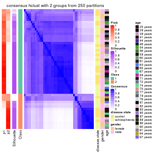
consensus_heatmap(res, k = 3)
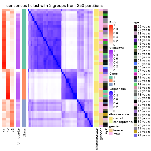
consensus_heatmap(res, k = 4)
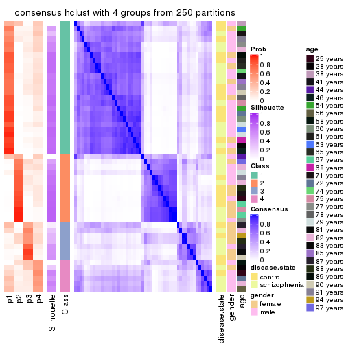
consensus_heatmap(res, k = 5)
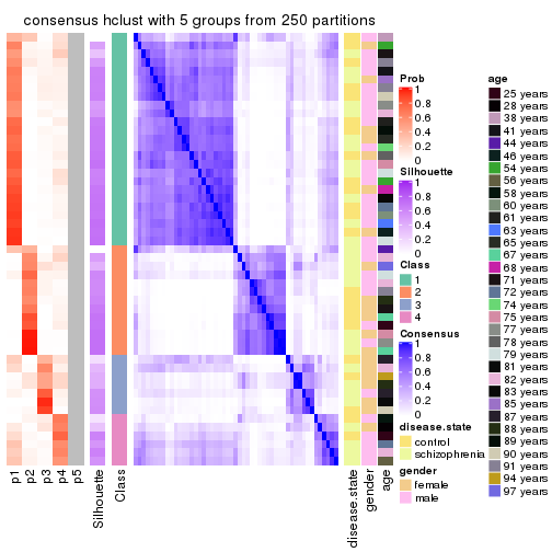
consensus_heatmap(res, k = 6)
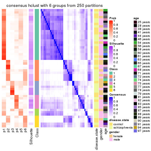
Heatmaps for the membership of samples in all partitions to see how consistent they are:
membership_heatmap(res, k = 2)
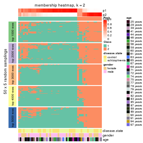
membership_heatmap(res, k = 3)
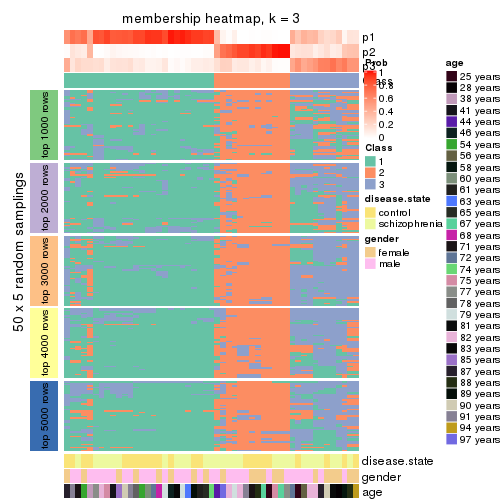
membership_heatmap(res, k = 4)
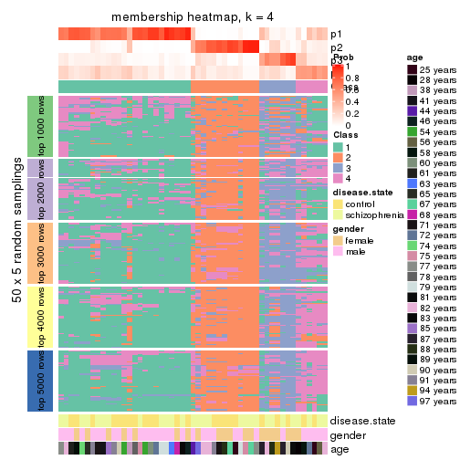
membership_heatmap(res, k = 5)
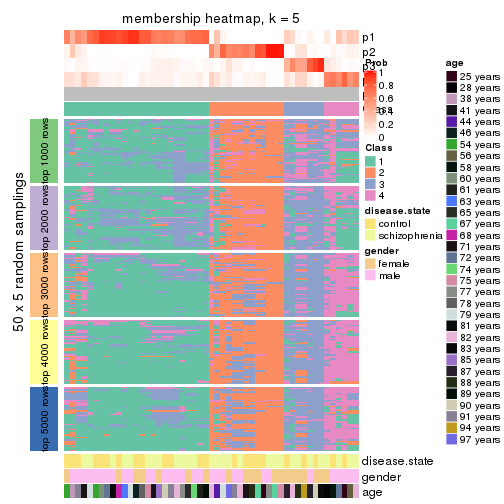
membership_heatmap(res, k = 6)
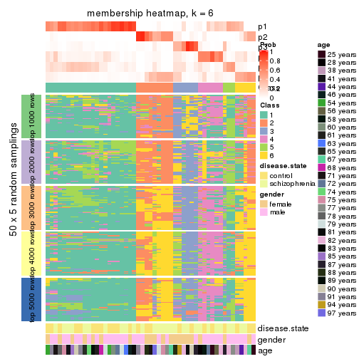
As soon as we have had the classes for columns, we can look for signatures which are significantly different between classes which can be candidate marks for certain classes. Following are the heatmaps for signatures.
Signature heatmaps where rows are scaled:
get_signatures(res, k = 2)
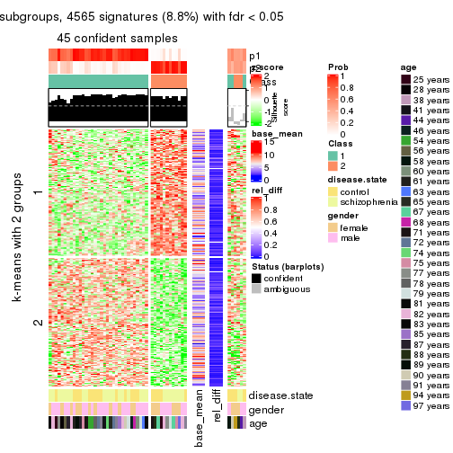
get_signatures(res, k = 3)
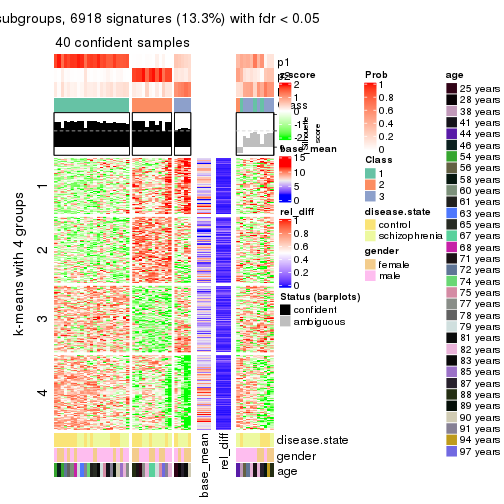
get_signatures(res, k = 4)
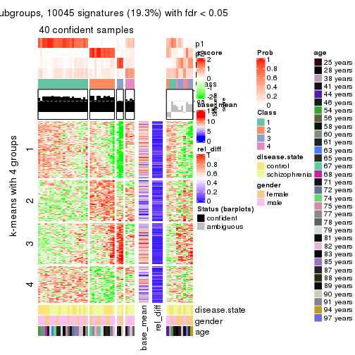
get_signatures(res, k = 5)
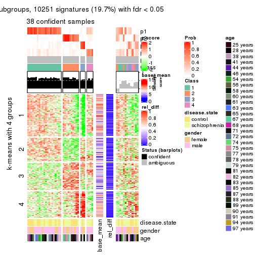
get_signatures(res, k = 6)
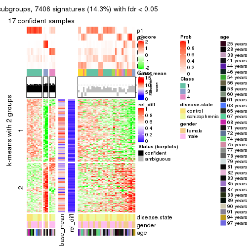
Signature heatmaps where rows are not scaled:
get_signatures(res, k = 2, scale_rows = FALSE)
get_signatures(res, k = 3, scale_rows = FALSE)
get_signatures(res, k = 4, scale_rows = FALSE)
get_signatures(res, k = 5, scale_rows = FALSE)
get_signatures(res, k = 6, scale_rows = FALSE)
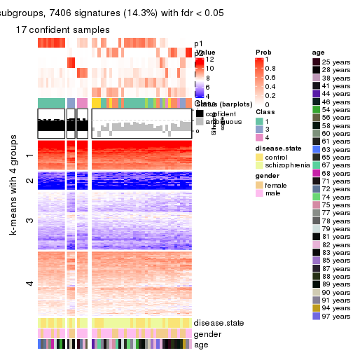
Compare the overlap of signatures from different k:
compare_signatures(res)
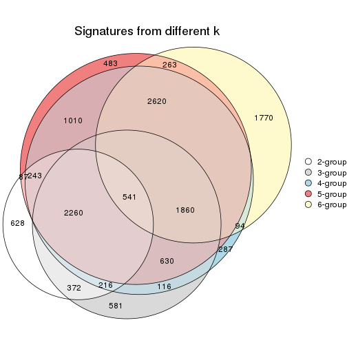
get_signature() returns a data frame invisibly. TO get the list of signatures, the function
call should be assigned to a variable explicitly. In following code, if plot argument is set
to FALSE, no heatmap is plotted while only the differential analysis is performed.
# code only for demonstration
tb = get_signature(res, k = ..., plot = FALSE)
An example of the output of tb is:
#>   which_row         fdr    mean_1    mean_2 scaled_mean_1 scaled_mean_2 km
#> 1        38 0.042760348  8.373488  9.131774    -0.5533452     0.5164555  1
#> 2        40 0.018707592  7.106213  8.469186    -0.6173731     0.5762149  1
#> 3        55 0.019134737 10.221463 11.207825    -0.6159697     0.5749050  1
#> 4        59 0.006059896  5.921854  7.869574    -0.6899429     0.6439467  1
#> 5        60 0.018055526  8.928898 10.211722    -0.6204761     0.5791110  1
#> 6        98 0.009384629 15.714769 14.887706     0.6635654    -0.6193277  2
...
The columns in tb are:
which_row: row indices corresponding to the input matrix.fdr: FDR for the differential test. mean_x: The mean value in group x.scaled_mean_x: The mean value in group x after rows are scaled.km: Row groups if k-means clustering is applied to rows.UMAP plot which shows how samples are separated.
dimension_reduction(res, k = 2, method = "UMAP")

dimension_reduction(res, k = 3, method = "UMAP")
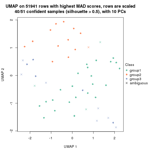
dimension_reduction(res, k = 4, method = "UMAP")
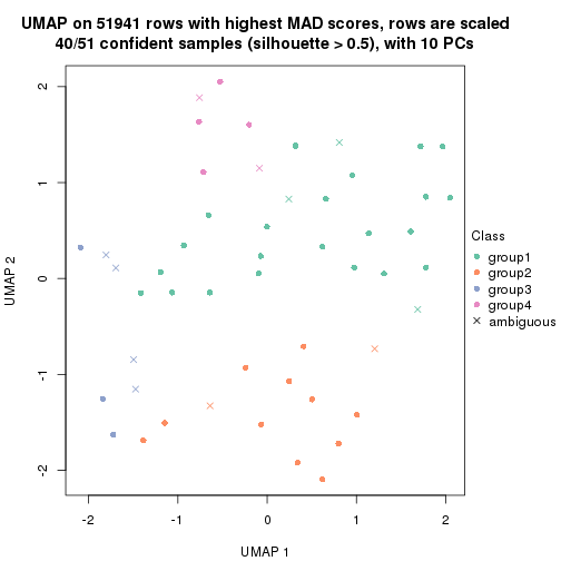
dimension_reduction(res, k = 5, method = "UMAP")
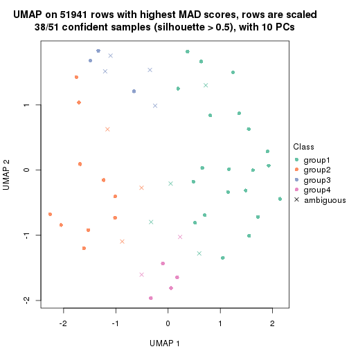
dimension_reduction(res, k = 6, method = "UMAP")
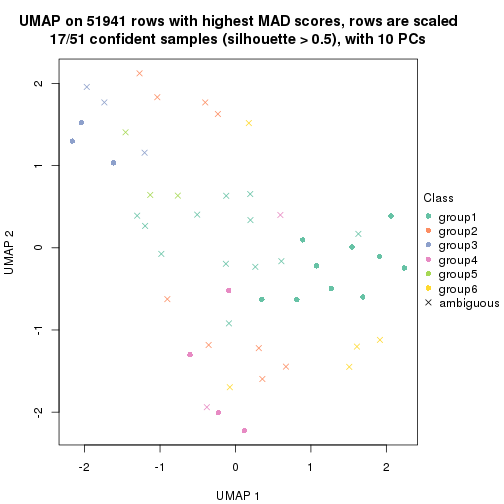
Following heatmap shows how subgroups are split when increasing k:
collect_classes(res)
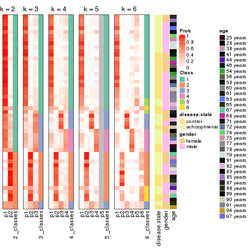
Test correlation between subgroups and known annotations. If the known annotation is numeric, one-way ANOVA test is applied, and if the known annotation is discrete, chi-squared contingency table test is applied.
test_to_known_factors(res)
#>             n disease.state(p) gender(p) age(p) k
#> MAD:hclust 45            1.000     0.502  0.790 2
#> MAD:hclust 40            0.787     0.331  0.465 3
#> MAD:hclust 40            0.793     0.200  0.592 4
#> MAD:hclust 38            0.734     0.180  0.604 5
#> MAD:hclust 17            0.432     0.159  0.414 6
If matrix rows can be associated to genes, consider to use functional_enrichment(res,
...) to perform function enrichment for the signature genes. See this vignette for more detailed explanations.
The object with results only for a single top-value method and a single partition method can be extracted as:
res = res_list["MAD", "kmeans"]
# you can also extract it by
# res = res_list["MAD:kmeans"]
A summary of res and all the functions that can be applied to it:
res
#> A 'ConsensusPartition' object with k = 2, 3, 4, 5, 6.
#>   On a matrix with 51941 rows and 51 columns.
#>   Top rows (1000, 2000, 3000, 4000, 5000) are extracted by 'MAD' method.
#>   Subgroups are detected by 'kmeans' method.
#>   Performed in total 1250 partitions by row resampling.
#>   Best k for subgroups seems to be 2.
#>
#> Following methods can be applied to this 'ConsensusPartition' object:
#>  [1] "cola_report"             "collect_classes"         "collect_plots"
#>  [4] "collect_stats"           "colnames"                "compare_signatures"
#>  [7] "consensus_heatmap"       "dimension_reduction"     "functional_enrichment"
#> [10] "get_anno_col"            "get_anno"                "get_classes"
#> [13] "get_consensus"           "get_matrix"              "get_membership"
#> [16] "get_param"               "get_signatures"          "get_stats"
#> [19] "is_best_k"               "is_stable_k"             "membership_heatmap"
#> [22] "ncol"                    "nrow"                    "plot_ecdf"
#> [25] "rownames"                "select_partition_number" "show"
#> [28] "suggest_best_k"          "test_to_known_factors"
collect_plots() function collects all the plots made from res for all k (number of partitions)
into one single page to provide an easy and fast comparison between different k.
collect_plots(res)
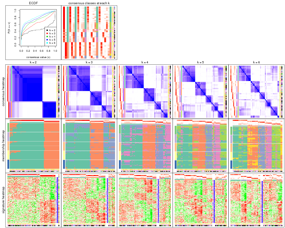
The plots are:
k and the heatmap of
predicted classes for each k.k.k.k.All the plots in panels can be made by individual functions and they are plotted later in this section.
select_partition_number() produces several plots showing different
statistics for choosing “optimized” k. There are following statistics:
k;k, the area increased is defined as \(A_k - A_{k-1}\).The detailed explanations of these statistics can be found in the cola vignette.
Generally speaking, lower PAC score, higher mean silhouette score or higher
concordance corresponds to better partition. Rand index and Jaccard index
measure how similar the current partition is compared to partition with k-1.
If they are too similar, we won't accept k is better than k-1.
select_partition_number(res)
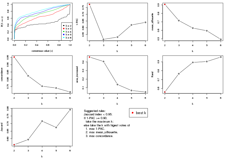
The numeric values for all these statistics can be obtained by get_stats().
get_stats(res)
#>   k 1-PAC mean_silhouette concordance area_increased  Rand Jaccard
#> 2 2 0.773           0.906       0.953         0.4571 0.561   0.561
#> 3 3 0.514           0.715       0.824         0.4055 0.766   0.595
#> 4 4 0.531           0.627       0.753         0.1370 0.893   0.716
#> 5 5 0.621           0.595       0.740         0.0675 0.904   0.675
#> 6 6 0.640           0.494       0.713         0.0496 0.954   0.792
suggest_best_k() suggests the best \(k\) based on these statistics. The rules are as follows:
suggest_best_k(res)
#> [1] 2
Following shows the table of the partitions (You need to click the show/hide
code output link to see it). The membership matrix (columns with name p*)
is inferred by
clue::cl_consensus()
function with the SE method. Basically the value in the membership matrix
represents the probability to belong to a certain group. The finall class
label for an item is determined with the group with highest probability it
belongs to.
In get_classes() function, the entropy is calculated from the membership
matrix and the silhouette score is calculated from the consensus matrix.
cbind(get_classes(res, k = 2), get_membership(res, k = 2))
#>           class entropy silhouette    p1    p2
#> GSM439800     1  0.6973      0.798 0.812 0.188
#> GSM439790     1  0.0000      0.935 1.000 0.000
#> GSM439827     2  0.0376      0.983 0.004 0.996
#> GSM439811     2  0.0376      0.983 0.004 0.996
#> GSM439795     1  0.9866      0.352 0.568 0.432
#> GSM439805     1  0.2948      0.913 0.948 0.052
#> GSM439781     1  0.0000      0.935 1.000 0.000
#> GSM439807     1  0.8555      0.676 0.720 0.280
#> GSM439820     2  0.0000      0.982 0.000 1.000
#> GSM439784     1  0.0000      0.935 1.000 0.000
#> GSM439824     2  0.0672      0.980 0.008 0.992
#> GSM439794     1  0.7528      0.768 0.784 0.216
#> GSM439809     1  0.0000      0.935 1.000 0.000
#> GSM439785     1  0.2778      0.914 0.952 0.048
#> GSM439803     1  0.3431      0.905 0.936 0.064
#> GSM439778     1  0.0000      0.935 1.000 0.000
#> GSM439791     1  0.0000      0.935 1.000 0.000
#> GSM439786     1  0.0376      0.934 0.996 0.004
#> GSM439828     2  0.0376      0.983 0.004 0.996
#> GSM439806     1  0.0000      0.935 1.000 0.000
#> GSM439815     1  0.0000      0.935 1.000 0.000
#> GSM439817     2  0.0376      0.983 0.004 0.996
#> GSM439796     1  0.7602      0.764 0.780 0.220
#> GSM439798     1  0.0376      0.934 0.996 0.004
#> GSM439821     2  0.0000      0.982 0.000 1.000
#> GSM439823     2  0.0376      0.983 0.004 0.996
#> GSM439813     1  0.0000      0.935 1.000 0.000
#> GSM439801     1  0.9286      0.564 0.656 0.344
#> GSM439810     1  0.0000      0.935 1.000 0.000
#> GSM439783     1  0.0000      0.935 1.000 0.000
#> GSM439826     2  0.0376      0.983 0.004 0.996
#> GSM439812     1  0.0000      0.935 1.000 0.000
#> GSM439818     2  0.0376      0.983 0.004 0.996
#> GSM439792     1  0.0000      0.935 1.000 0.000
#> GSM439802     1  0.0376      0.934 0.996 0.004
#> GSM439825     2  0.0376      0.983 0.004 0.996
#> GSM439780     1  0.0376      0.934 0.996 0.004
#> GSM439787     2  0.7299      0.709 0.204 0.796
#> GSM439808     2  0.0000      0.982 0.000 1.000
#> GSM439804     1  0.6148      0.836 0.848 0.152
#> GSM439822     2  0.0376      0.983 0.004 0.996
#> GSM439816     1  0.5059      0.871 0.888 0.112
#> GSM439789     1  0.0000      0.935 1.000 0.000
#> GSM439799     2  0.0000      0.982 0.000 1.000
#> GSM439814     1  0.0000      0.935 1.000 0.000
#> GSM439782     1  0.0000      0.935 1.000 0.000
#> GSM439779     1  0.0000      0.935 1.000 0.000
#> GSM439793     1  0.0376      0.934 0.996 0.004
#> GSM439788     1  0.0000      0.935 1.000 0.000
#> GSM439797     1  0.2603      0.916 0.956 0.044
#> GSM439819     2  0.0000      0.982 0.000 1.000
cbind(get_classes(res, k = 3), get_membership(res, k = 3))
#>           class entropy silhouette    p1    p2    p3
#> GSM439800     3  0.5506      0.604 0.220 0.016 0.764
#> GSM439790     1  0.4291      0.783 0.820 0.000 0.180
#> GSM439827     2  0.0000      0.884 0.000 1.000 0.000
#> GSM439811     2  0.0000      0.884 0.000 1.000 0.000
#> GSM439795     3  0.4683      0.614 0.024 0.140 0.836
#> GSM439805     3  0.5222      0.614 0.144 0.040 0.816
#> GSM439781     1  0.5517      0.701 0.728 0.004 0.268
#> GSM439807     3  0.5524      0.606 0.040 0.164 0.796
#> GSM439820     2  0.2165      0.859 0.000 0.936 0.064
#> GSM439784     1  0.3129      0.818 0.904 0.008 0.088
#> GSM439824     2  0.5180      0.768 0.032 0.812 0.156
#> GSM439794     3  0.7773      0.520 0.316 0.072 0.612
#> GSM439809     1  0.0424      0.835 0.992 0.000 0.008
#> GSM439785     1  0.6496      0.651 0.736 0.056 0.208
#> GSM439803     3  0.7831      0.363 0.404 0.056 0.540
#> GSM439778     1  0.1860      0.835 0.948 0.000 0.052
#> GSM439791     1  0.0424      0.836 0.992 0.000 0.008
#> GSM439786     1  0.5690      0.671 0.708 0.004 0.288
#> GSM439828     2  0.0424      0.884 0.000 0.992 0.008
#> GSM439806     1  0.1643      0.834 0.956 0.000 0.044
#> GSM439815     1  0.2261      0.814 0.932 0.000 0.068
#> GSM439817     2  0.1031      0.884 0.000 0.976 0.024
#> GSM439796     3  0.7961      0.494 0.336 0.076 0.588
#> GSM439798     1  0.5690      0.671 0.708 0.004 0.288
#> GSM439821     2  0.2261      0.862 0.000 0.932 0.068
#> GSM439823     2  0.1753      0.875 0.000 0.952 0.048
#> GSM439813     1  0.0892      0.833 0.980 0.000 0.020
#> GSM439801     3  0.4810      0.614 0.028 0.140 0.832
#> GSM439810     1  0.0592      0.834 0.988 0.000 0.012
#> GSM439783     1  0.3192      0.773 0.888 0.000 0.112
#> GSM439826     2  0.3752      0.816 0.000 0.856 0.144
#> GSM439812     1  0.0747      0.832 0.984 0.000 0.016
#> GSM439818     2  0.3482      0.864 0.000 0.872 0.128
#> GSM439792     1  0.0747      0.836 0.984 0.000 0.016
#> GSM439802     3  0.5621      0.391 0.308 0.000 0.692
#> GSM439825     2  0.2261      0.878 0.000 0.932 0.068
#> GSM439780     1  0.4178      0.779 0.828 0.000 0.172
#> GSM439787     3  0.5305      0.576 0.020 0.192 0.788
#> GSM439808     2  0.6204      0.231 0.000 0.576 0.424
#> GSM439804     3  0.8201      0.376 0.400 0.076 0.524
#> GSM439822     2  0.3686      0.818 0.000 0.860 0.140
#> GSM439816     1  0.7107      0.483 0.712 0.092 0.196
#> GSM439789     1  0.3412      0.737 0.876 0.000 0.124
#> GSM439799     3  0.5882      0.249 0.000 0.348 0.652
#> GSM439814     1  0.0747      0.829 0.984 0.000 0.016
#> GSM439782     1  0.2165      0.833 0.936 0.000 0.064
#> GSM439779     1  0.0424      0.832 0.992 0.000 0.008
#> GSM439793     1  0.5365      0.713 0.744 0.004 0.252
#> GSM439788     1  0.5016      0.725 0.760 0.000 0.240
#> GSM439797     1  0.7189      0.604 0.656 0.052 0.292
#> GSM439819     2  0.2165      0.861 0.000 0.936 0.064
cbind(get_classes(res, k = 4), get_membership(res, k = 4))
#>           class entropy silhouette    p1    p2    p3    p4
#> GSM439800     4  0.6646     0.1296 0.048 0.016 0.444 0.492
#> GSM439790     1  0.6783     0.5595 0.616 0.004 0.144 0.236
#> GSM439827     2  0.0707     0.8801 0.000 0.980 0.000 0.020
#> GSM439811     2  0.0895     0.8792 0.000 0.976 0.004 0.020
#> GSM439795     3  0.1247     0.7360 0.004 0.016 0.968 0.012
#> GSM439805     3  0.2861     0.6777 0.016 0.000 0.888 0.096
#> GSM439781     1  0.7693     0.4450 0.488 0.004 0.232 0.276
#> GSM439807     3  0.1994     0.7346 0.004 0.052 0.936 0.008
#> GSM439820     2  0.2859     0.8283 0.000 0.880 0.112 0.008
#> GSM439784     1  0.6143     0.5975 0.692 0.012 0.092 0.204
#> GSM439824     2  0.4631     0.7189 0.008 0.728 0.004 0.260
#> GSM439794     4  0.6835     0.6025 0.096 0.040 0.200 0.664
#> GSM439809     1  0.1209     0.6940 0.964 0.000 0.004 0.032
#> GSM439785     4  0.7279     0.2482 0.308 0.028 0.096 0.568
#> GSM439803     4  0.6710     0.6423 0.144 0.028 0.152 0.676
#> GSM439778     1  0.3647     0.6774 0.852 0.000 0.040 0.108
#> GSM439791     1  0.1389     0.6974 0.952 0.000 0.000 0.048
#> GSM439786     1  0.7662     0.4536 0.496 0.004 0.236 0.264
#> GSM439828     2  0.0895     0.8799 0.000 0.976 0.004 0.020
#> GSM439806     1  0.2708     0.6937 0.904 0.004 0.016 0.076
#> GSM439815     1  0.3958     0.6072 0.836 0.000 0.052 0.112
#> GSM439817     2  0.1256     0.8787 0.000 0.964 0.008 0.028
#> GSM439796     4  0.6941     0.6343 0.124 0.040 0.172 0.664
#> GSM439798     1  0.7723     0.4388 0.484 0.004 0.248 0.264
#> GSM439821     2  0.4231     0.8371 0.000 0.824 0.096 0.080
#> GSM439823     2  0.1557     0.8762 0.000 0.944 0.000 0.056
#> GSM439813     1  0.2048     0.6716 0.928 0.000 0.008 0.064
#> GSM439801     3  0.1745     0.7335 0.008 0.020 0.952 0.020
#> GSM439810     1  0.1398     0.6852 0.956 0.000 0.004 0.040
#> GSM439783     1  0.4914     0.4051 0.676 0.000 0.012 0.312
#> GSM439826     2  0.3681     0.8341 0.000 0.816 0.008 0.176
#> GSM439812     1  0.2124     0.6697 0.924 0.000 0.008 0.068
#> GSM439818     2  0.4238     0.8479 0.000 0.796 0.028 0.176
#> GSM439792     1  0.3271     0.6888 0.856 0.000 0.012 0.132
#> GSM439802     3  0.5160     0.5100 0.136 0.000 0.760 0.104
#> GSM439825     2  0.3606     0.8612 0.000 0.844 0.024 0.132
#> GSM439780     1  0.4840     0.6534 0.784 0.000 0.100 0.116
#> GSM439787     3  0.2676     0.7192 0.000 0.092 0.896 0.012
#> GSM439808     3  0.5172     0.2829 0.000 0.404 0.588 0.008
#> GSM439804     4  0.6832     0.6427 0.132 0.040 0.152 0.676
#> GSM439822     2  0.3893     0.8334 0.000 0.796 0.008 0.196
#> GSM439816     4  0.7031     0.3576 0.380 0.088 0.012 0.520
#> GSM439789     1  0.4584     0.3584 0.696 0.000 0.004 0.300
#> GSM439799     3  0.7169     0.2193 0.000 0.152 0.516 0.332
#> GSM439814     1  0.2124     0.6697 0.924 0.000 0.008 0.068
#> GSM439782     1  0.3999     0.6669 0.824 0.000 0.036 0.140
#> GSM439779     1  0.1398     0.6912 0.956 0.000 0.004 0.040
#> GSM439793     1  0.7579     0.4683 0.512 0.004 0.228 0.256
#> GSM439788     1  0.7267     0.5098 0.556 0.004 0.180 0.260
#> GSM439797     4  0.7317     0.0964 0.296 0.016 0.128 0.560
#> GSM439819     2  0.3354     0.8428 0.000 0.872 0.084 0.044
cbind(get_classes(res, k = 5), get_membership(res, k = 5))
#>           class entropy silhouette    p1    p2    p3    p4    p5
#> GSM439800     4  0.5757     0.3731 0.040 0.008 0.324 0.604 0.024
#> GSM439790     5  0.6061     0.6316 0.376 0.000 0.052 0.036 0.536
#> GSM439827     2  0.1179     0.8011 0.000 0.964 0.004 0.016 0.016
#> GSM439811     2  0.1524     0.8000 0.000 0.952 0.016 0.016 0.016
#> GSM439795     3  0.1267     0.8303 0.004 0.000 0.960 0.012 0.024
#> GSM439805     3  0.2050     0.8166 0.008 0.000 0.920 0.008 0.064
#> GSM439781     5  0.6577     0.7619 0.284 0.008 0.096 0.036 0.576
#> GSM439807     3  0.1603     0.8178 0.004 0.004 0.948 0.012 0.032
#> GSM439820     2  0.3610     0.7471 0.000 0.844 0.088 0.020 0.048
#> GSM439784     1  0.6284    -0.2422 0.520 0.008 0.036 0.048 0.388
#> GSM439824     2  0.4910     0.5887 0.004 0.672 0.000 0.276 0.048
#> GSM439794     4  0.3561     0.7169 0.072 0.008 0.048 0.856 0.016
#> GSM439809     1  0.0880     0.6511 0.968 0.000 0.000 0.000 0.032
#> GSM439785     4  0.6919     0.0591 0.116 0.028 0.012 0.508 0.336
#> GSM439803     4  0.3503     0.7154 0.076 0.008 0.024 0.860 0.032
#> GSM439778     1  0.5413     0.4381 0.664 0.000 0.012 0.080 0.244
#> GSM439791     1  0.3489     0.6048 0.820 0.000 0.000 0.036 0.144
#> GSM439786     5  0.6092     0.7580 0.268 0.000 0.096 0.028 0.608
#> GSM439828     2  0.1186     0.7983 0.000 0.964 0.008 0.008 0.020
#> GSM439806     1  0.3365     0.5538 0.808 0.008 0.000 0.004 0.180
#> GSM439815     1  0.3300     0.6000 0.856 0.000 0.024 0.100 0.020
#> GSM439817     2  0.2673     0.7776 0.000 0.900 0.028 0.024 0.048
#> GSM439796     4  0.3496     0.7176 0.072 0.012 0.044 0.860 0.012
#> GSM439798     5  0.5977     0.7554 0.268 0.000 0.108 0.016 0.608
#> GSM439821     2  0.6102     0.7281 0.000 0.644 0.068 0.068 0.220
#> GSM439823     2  0.2943     0.7827 0.000 0.880 0.008 0.052 0.060
#> GSM439813     1  0.0798     0.6589 0.976 0.000 0.000 0.016 0.008
#> GSM439801     3  0.2120     0.8279 0.004 0.004 0.924 0.020 0.048
#> GSM439810     1  0.0579     0.6612 0.984 0.000 0.000 0.008 0.008
#> GSM439783     1  0.6040     0.2979 0.504 0.000 0.000 0.372 0.124
#> GSM439826     2  0.4922     0.7575 0.000 0.716 0.000 0.128 0.156
#> GSM439812     1  0.1012     0.6593 0.968 0.000 0.000 0.020 0.012
#> GSM439818     2  0.5869     0.7251 0.000 0.600 0.004 0.128 0.268
#> GSM439792     1  0.4369     0.5278 0.740 0.000 0.000 0.052 0.208
#> GSM439802     3  0.4455     0.6496 0.036 0.000 0.736 0.008 0.220
#> GSM439825     2  0.5577     0.7375 0.000 0.636 0.008 0.092 0.264
#> GSM439780     1  0.5068    -0.0579 0.580 0.000 0.032 0.004 0.384
#> GSM439787     3  0.1748     0.8224 0.004 0.016 0.944 0.008 0.028
#> GSM439808     3  0.5492     0.4067 0.000 0.324 0.612 0.024 0.040
#> GSM439804     4  0.3487     0.7189 0.080 0.012 0.032 0.860 0.016
#> GSM439822     2  0.5733     0.7307 0.000 0.620 0.000 0.160 0.220
#> GSM439816     4  0.6476     0.3147 0.316 0.064 0.000 0.556 0.064
#> GSM439789     1  0.4663     0.2895 0.604 0.000 0.000 0.376 0.020
#> GSM439799     4  0.7161     0.0685 0.000 0.124 0.356 0.460 0.060
#> GSM439814     1  0.0898     0.6591 0.972 0.000 0.000 0.020 0.008
#> GSM439782     1  0.5393     0.2780 0.608 0.000 0.000 0.080 0.312
#> GSM439779     1  0.3551     0.6163 0.820 0.000 0.000 0.044 0.136
#> GSM439793     5  0.6597     0.7073 0.360 0.008 0.088 0.028 0.516
#> GSM439788     5  0.5900     0.7126 0.372 0.000 0.076 0.012 0.540
#> GSM439797     5  0.7305     0.2415 0.100 0.024 0.044 0.348 0.484
#> GSM439819     2  0.4893     0.7591 0.000 0.760 0.068 0.040 0.132
cbind(get_classes(res, k = 6), get_membership(res, k = 6))
#>           class entropy silhouette    p1    p2    p3    p4    p5    p6
#> GSM439800     4  0.4909     0.5510 0.004 0.000 0.188 0.692 0.012 0.104
#> GSM439790     5  0.5295     0.5411 0.208 0.000 0.020 0.004 0.656 0.112
#> GSM439827     2  0.1523     0.4609 0.000 0.940 0.000 0.008 0.008 0.044
#> GSM439811     2  0.1799     0.4610 0.000 0.928 0.004 0.008 0.008 0.052
#> GSM439795     3  0.1616     0.7763 0.000 0.000 0.940 0.028 0.020 0.012
#> GSM439805     3  0.2663     0.7636 0.000 0.000 0.876 0.028 0.084 0.012
#> GSM439781     5  0.3383     0.7223 0.100 0.012 0.016 0.000 0.840 0.032
#> GSM439807     3  0.3883     0.7525 0.004 0.008 0.816 0.040 0.032 0.100
#> GSM439820     2  0.4818     0.3916 0.000 0.748 0.080 0.028 0.024 0.120
#> GSM439784     5  0.5040     0.4246 0.304 0.028 0.000 0.008 0.628 0.032
#> GSM439824     2  0.6057     0.0269 0.008 0.580 0.004 0.228 0.020 0.160
#> GSM439794     4  0.1768     0.7736 0.044 0.000 0.012 0.932 0.008 0.004
#> GSM439809     1  0.2237     0.6787 0.896 0.000 0.000 0.000 0.068 0.036
#> GSM439785     5  0.5619     0.1308 0.032 0.012 0.000 0.444 0.472 0.040
#> GSM439803     4  0.2178     0.7707 0.056 0.000 0.008 0.912 0.012 0.012
#> GSM439778     1  0.5856     0.4596 0.560 0.000 0.004 0.032 0.304 0.100
#> GSM439791     1  0.3791     0.6371 0.760 0.000 0.000 0.008 0.200 0.032
#> GSM439786     5  0.3857     0.7046 0.064 0.000 0.032 0.004 0.812 0.088
#> GSM439828     2  0.0291     0.4770 0.000 0.992 0.000 0.000 0.004 0.004
#> GSM439806     1  0.4228     0.5773 0.704 0.012 0.000 0.000 0.252 0.032
#> GSM439815     1  0.3861     0.6154 0.820 0.000 0.048 0.060 0.008 0.064
#> GSM439817     2  0.3261     0.4640 0.000 0.852 0.016 0.024 0.020 0.088
#> GSM439796     4  0.1542     0.7751 0.052 0.000 0.008 0.936 0.004 0.000
#> GSM439798     5  0.3562     0.7102 0.064 0.000 0.032 0.000 0.828 0.076
#> GSM439821     2  0.5593    -0.4183 0.000 0.496 0.068 0.012 0.012 0.412
#> GSM439823     2  0.3458     0.4555 0.000 0.840 0.012 0.048 0.016 0.084
#> GSM439813     1  0.1296     0.6712 0.948 0.000 0.000 0.004 0.004 0.044
#> GSM439801     3  0.2798     0.7733 0.000 0.004 0.880 0.036 0.060 0.020
#> GSM439810     1  0.1138     0.6852 0.960 0.000 0.004 0.000 0.024 0.012
#> GSM439783     1  0.6818     0.4239 0.488 0.000 0.004 0.248 0.188 0.072
#> GSM439826     2  0.5284    -0.4294 0.000 0.572 0.000 0.084 0.012 0.332
#> GSM439812     1  0.1296     0.6712 0.948 0.000 0.000 0.004 0.004 0.044
#> GSM439818     6  0.5055     0.7856 0.000 0.420 0.000 0.056 0.008 0.516
#> GSM439792     1  0.5029     0.5019 0.620 0.000 0.004 0.016 0.308 0.052
#> GSM439802     3  0.5460     0.5576 0.040 0.000 0.664 0.004 0.176 0.116
#> GSM439825     6  0.4752     0.7835 0.000 0.448 0.008 0.024 0.004 0.516
#> GSM439780     1  0.5949     0.1277 0.472 0.000 0.036 0.000 0.396 0.096
#> GSM439787     3  0.3983     0.7599 0.000 0.028 0.820 0.044 0.044 0.064
#> GSM439808     3  0.6975     0.3146 0.000 0.292 0.484 0.052 0.032 0.140
#> GSM439804     4  0.1606     0.7747 0.056 0.000 0.004 0.932 0.008 0.000
#> GSM439822     2  0.5272    -0.6940 0.000 0.484 0.000 0.084 0.004 0.428
#> GSM439816     4  0.7547     0.1308 0.328 0.072 0.004 0.424 0.056 0.116
#> GSM439789     1  0.4766     0.5035 0.676 0.000 0.004 0.256 0.040 0.024
#> GSM439799     4  0.6309     0.4399 0.000 0.092 0.152 0.620 0.020 0.116
#> GSM439814     1  0.1340     0.6741 0.948 0.000 0.000 0.004 0.008 0.040
#> GSM439782     1  0.6839     0.2061 0.432 0.000 0.016 0.056 0.364 0.132
#> GSM439779     1  0.3890     0.6341 0.752 0.000 0.000 0.008 0.204 0.036
#> GSM439793     5  0.3531     0.7103 0.140 0.004 0.028 0.000 0.812 0.016
#> GSM439788     5  0.3348     0.7057 0.152 0.000 0.020 0.000 0.812 0.016
#> GSM439797     5  0.4065     0.6170 0.020 0.016 0.000 0.196 0.756 0.012
#> GSM439819     2  0.4848     0.1698 0.000 0.692 0.064 0.008 0.016 0.220
Heatmaps for the consensus matrix. It visualizes the probability of two samples to be in a same group.
consensus_heatmap(res, k = 2)
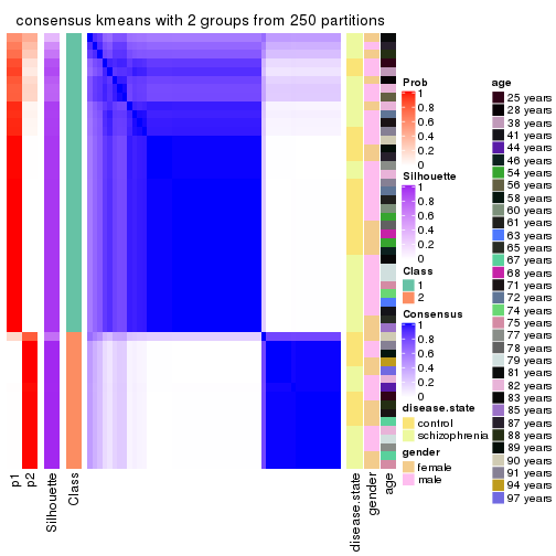
consensus_heatmap(res, k = 3)
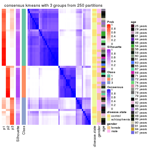
consensus_heatmap(res, k = 4)
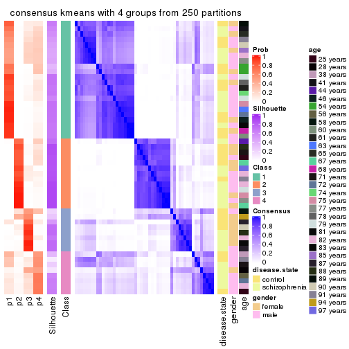
consensus_heatmap(res, k = 5)
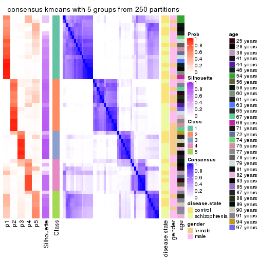
consensus_heatmap(res, k = 6)
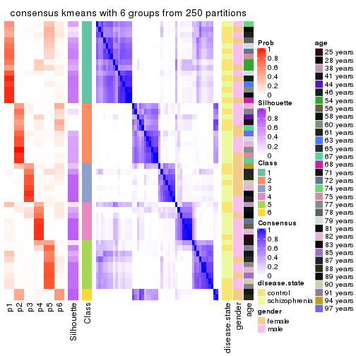
Heatmaps for the membership of samples in all partitions to see how consistent they are:
membership_heatmap(res, k = 2)
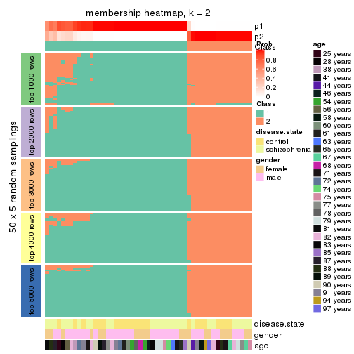
membership_heatmap(res, k = 3)
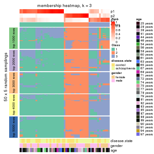
membership_heatmap(res, k = 4)
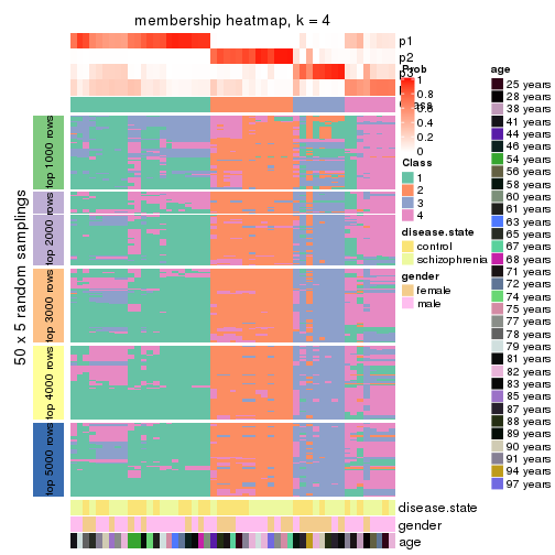
membership_heatmap(res, k = 5)
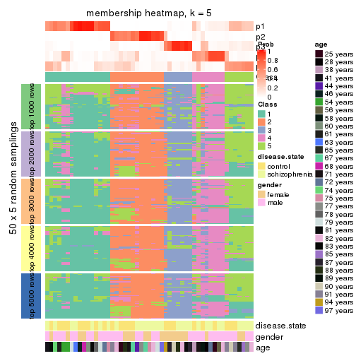
membership_heatmap(res, k = 6)
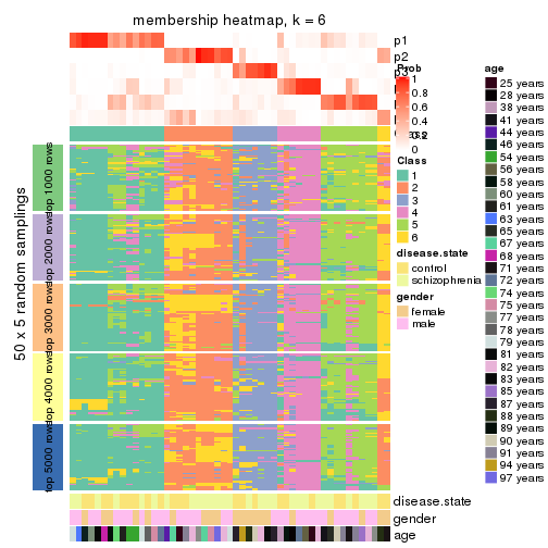
As soon as we have had the classes for columns, we can look for signatures which are significantly different between classes which can be candidate marks for certain classes. Following are the heatmaps for signatures.
Signature heatmaps where rows are scaled:
get_signatures(res, k = 2)
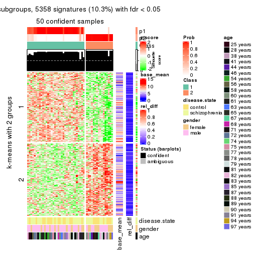
get_signatures(res, k = 3)
get_signatures(res, k = 4)
get_signatures(res, k = 5)
get_signatures(res, k = 6)
Signature heatmaps where rows are not scaled:
get_signatures(res, k = 2, scale_rows = FALSE)
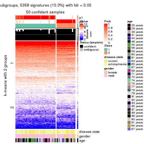
get_signatures(res, k = 3, scale_rows = FALSE)
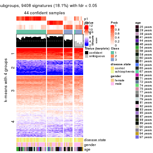
get_signatures(res, k = 4, scale_rows = FALSE)
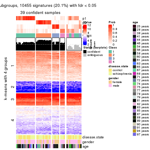
get_signatures(res, k = 5, scale_rows = FALSE)
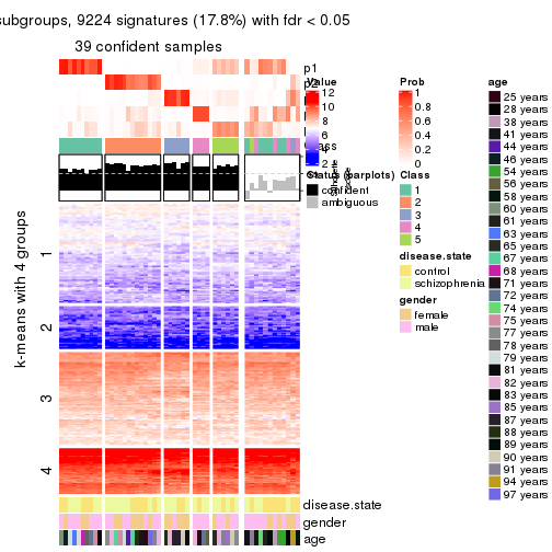
get_signatures(res, k = 6, scale_rows = FALSE)
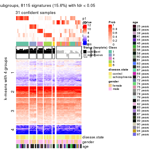
Compare the overlap of signatures from different k:
compare_signatures(res)
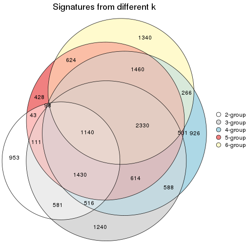
get_signature() returns a data frame invisibly. TO get the list of signatures, the function
call should be assigned to a variable explicitly. In following code, if plot argument is set
to FALSE, no heatmap is plotted while only the differential analysis is performed.
# code only for demonstration
tb = get_signature(res, k = ..., plot = FALSE)
An example of the output of tb is:
#>   which_row         fdr    mean_1    mean_2 scaled_mean_1 scaled_mean_2 km
#> 1        38 0.042760348  8.373488  9.131774    -0.5533452     0.5164555  1
#> 2        40 0.018707592  7.106213  8.469186    -0.6173731     0.5762149  1
#> 3        55 0.019134737 10.221463 11.207825    -0.6159697     0.5749050  1
#> 4        59 0.006059896  5.921854  7.869574    -0.6899429     0.6439467  1
#> 5        60 0.018055526  8.928898 10.211722    -0.6204761     0.5791110  1
#> 6        98 0.009384629 15.714769 14.887706     0.6635654    -0.6193277  2
...
The columns in tb are:
which_row: row indices corresponding to the input matrix.fdr: FDR for the differential test. mean_x: The mean value in group x.scaled_mean_x: The mean value in group x after rows are scaled.km: Row groups if k-means clustering is applied to rows.UMAP plot which shows how samples are separated.
dimension_reduction(res, k = 2, method = "UMAP")
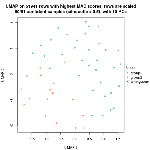
dimension_reduction(res, k = 3, method = "UMAP")
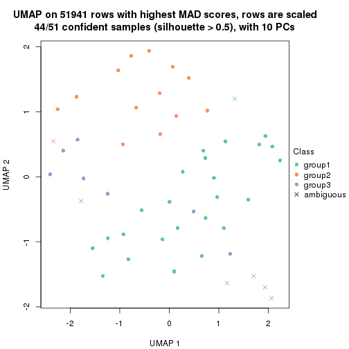
dimension_reduction(res, k = 4, method = "UMAP")
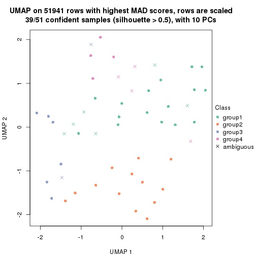
dimension_reduction(res, k = 5, method = "UMAP")
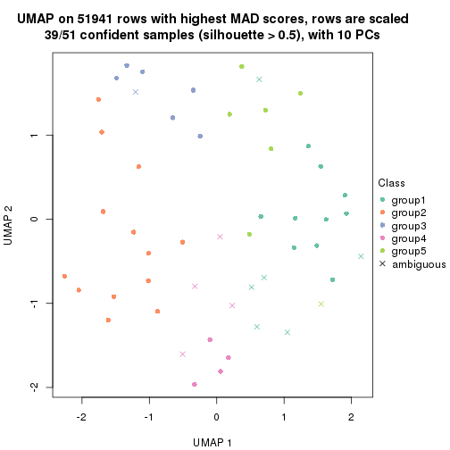
dimension_reduction(res, k = 6, method = "UMAP")
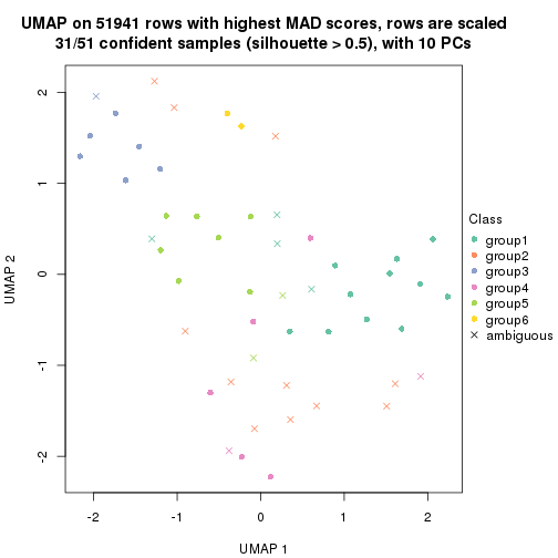
Following heatmap shows how subgroups are split when increasing k:
collect_classes(res)
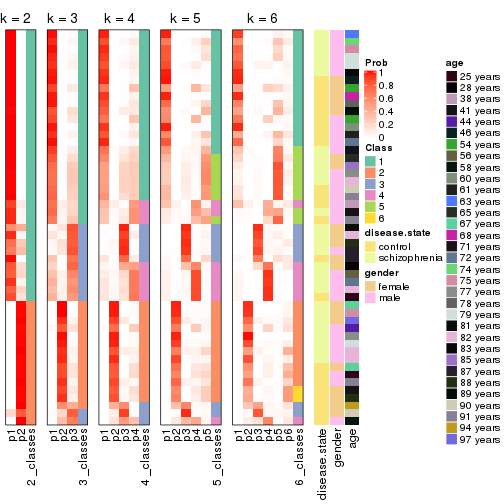
Test correlation between subgroups and known annotations. If the known annotation is numeric, one-way ANOVA test is applied, and if the known annotation is discrete, chi-squared contingency table test is applied.
test_to_known_factors(res)
#>             n disease.state(p) gender(p) age(p) k
#> MAD:kmeans 50            0.932    0.3751  0.787 2
#> MAD:kmeans 44            0.234    0.1216  0.593 3
#> MAD:kmeans 39            0.768    0.0461  0.558 4
#> MAD:kmeans 39            0.909    0.0911  0.475 5
#> MAD:kmeans 31            0.348    0.0505  0.316 6
If matrix rows can be associated to genes, consider to use functional_enrichment(res,
...) to perform function enrichment for the signature genes. See this vignette for more detailed explanations.
The object with results only for a single top-value method and a single partition method can be extracted as:
res = res_list["MAD", "skmeans"]
# you can also extract it by
# res = res_list["MAD:skmeans"]
A summary of res and all the functions that can be applied to it:
res
#> A 'ConsensusPartition' object with k = 2, 3, 4, 5, 6.
#>   On a matrix with 51941 rows and 51 columns.
#>   Top rows (1000, 2000, 3000, 4000, 5000) are extracted by 'MAD' method.
#>   Subgroups are detected by 'skmeans' method.
#>   Performed in total 1250 partitions by row resampling.
#>   Best k for subgroups seems to be 2.
#>
#> Following methods can be applied to this 'ConsensusPartition' object:
#>  [1] "cola_report"             "collect_classes"         "collect_plots"
#>  [4] "collect_stats"           "colnames"                "compare_signatures"
#>  [7] "consensus_heatmap"       "dimension_reduction"     "functional_enrichment"
#> [10] "get_anno_col"            "get_anno"                "get_classes"
#> [13] "get_consensus"           "get_matrix"              "get_membership"
#> [16] "get_param"               "get_signatures"          "get_stats"
#> [19] "is_best_k"               "is_stable_k"             "membership_heatmap"
#> [22] "ncol"                    "nrow"                    "plot_ecdf"
#> [25] "rownames"                "select_partition_number" "show"
#> [28] "suggest_best_k"          "test_to_known_factors"
collect_plots() function collects all the plots made from res for all k (number of partitions)
into one single page to provide an easy and fast comparison between different k.
collect_plots(res)
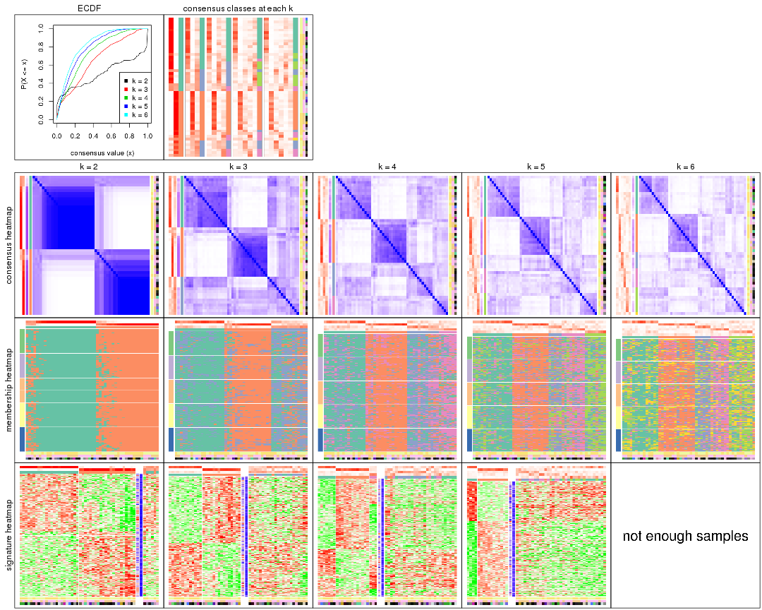
The plots are:
k and the heatmap of
predicted classes for each k.k.k.k.All the plots in panels can be made by individual functions and they are plotted later in this section.
select_partition_number() produces several plots showing different
statistics for choosing “optimized” k. There are following statistics:
k;k, the area increased is defined as \(A_k - A_{k-1}\).The detailed explanations of these statistics can be found in the cola vignette.
Generally speaking, lower PAC score, higher mean silhouette score or higher
concordance corresponds to better partition. Rand index and Jaccard index
measure how similar the current partition is compared to partition with k-1.
If they are too similar, we won't accept k is better than k-1.
select_partition_number(res)
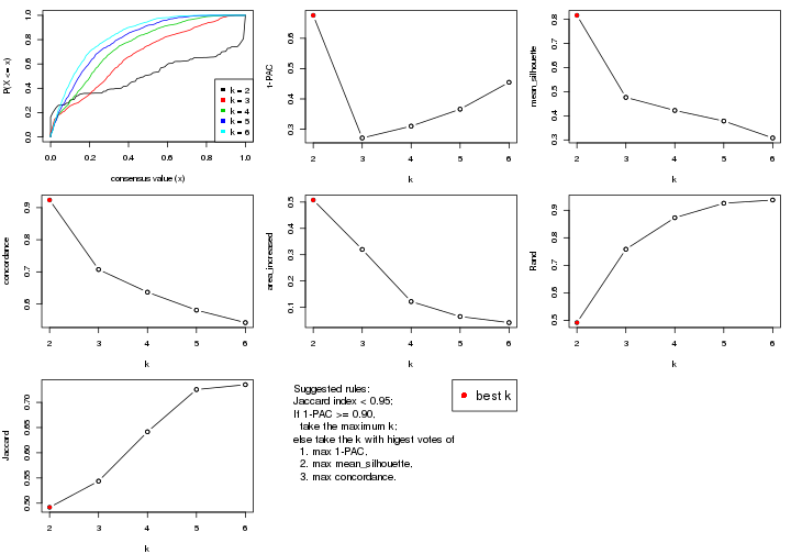
The numeric values for all these statistics can be obtained by get_stats().
get_stats(res)
#>   k 1-PAC mean_silhouette concordance area_increased  Rand Jaccard
#> 2 2 0.676           0.816       0.924         0.5078 0.492   0.492
#> 3 3 0.271           0.476       0.707         0.3199 0.758   0.544
#> 4 4 0.310           0.422       0.637         0.1219 0.873   0.642
#> 5 5 0.366           0.378       0.581         0.0649 0.925   0.725
#> 6 6 0.455           0.308       0.542         0.0417 0.937   0.735
suggest_best_k() suggests the best \(k\) based on these statistics. The rules are as follows:
suggest_best_k(res)
#> [1] 2
Following shows the table of the partitions (You need to click the show/hide
code output link to see it). The membership matrix (columns with name p*)
is inferred by
clue::cl_consensus()
function with the SE method. Basically the value in the membership matrix
represents the probability to belong to a certain group. The finall class
label for an item is determined with the group with highest probability it
belongs to.
In get_classes() function, the entropy is calculated from the membership
matrix and the silhouette score is calculated from the consensus matrix.
cbind(get_classes(res, k = 2), get_membership(res, k = 2))
#>           class entropy silhouette    p1    p2
#> GSM439800     2  0.8713      0.610 0.292 0.708
#> GSM439790     1  0.0000      0.912 1.000 0.000
#> GSM439827     2  0.0000      0.915 0.000 1.000
#> GSM439811     2  0.0000      0.915 0.000 1.000
#> GSM439795     2  0.3733      0.879 0.072 0.928
#> GSM439805     1  0.9896      0.208 0.560 0.440
#> GSM439781     1  0.4562      0.842 0.904 0.096
#> GSM439807     2  0.8386      0.645 0.268 0.732
#> GSM439820     2  0.0000      0.915 0.000 1.000
#> GSM439784     1  0.5946      0.793 0.856 0.144
#> GSM439824     2  0.1414      0.908 0.020 0.980
#> GSM439794     2  0.4562      0.863 0.096 0.904
#> GSM439809     1  0.0000      0.912 1.000 0.000
#> GSM439785     1  0.9896      0.218 0.560 0.440
#> GSM439803     1  0.9775      0.282 0.588 0.412
#> GSM439778     1  0.0000      0.912 1.000 0.000
#> GSM439791     1  0.0000      0.912 1.000 0.000
#> GSM439786     1  0.0000      0.912 1.000 0.000
#> GSM439828     2  0.0000      0.915 0.000 1.000
#> GSM439806     1  0.0000      0.912 1.000 0.000
#> GSM439815     1  0.1843      0.896 0.972 0.028
#> GSM439817     2  0.0376      0.914 0.004 0.996
#> GSM439796     2  0.5519      0.834 0.128 0.872
#> GSM439798     1  0.0672      0.909 0.992 0.008
#> GSM439821     2  0.0000      0.915 0.000 1.000
#> GSM439823     2  0.0000      0.915 0.000 1.000
#> GSM439813     1  0.0000      0.912 1.000 0.000
#> GSM439801     2  0.5408      0.837 0.124 0.876
#> GSM439810     1  0.0000      0.912 1.000 0.000
#> GSM439783     1  0.0938      0.907 0.988 0.012
#> GSM439826     2  0.0000      0.915 0.000 1.000
#> GSM439812     1  0.0000      0.912 1.000 0.000
#> GSM439818     2  0.0000      0.915 0.000 1.000
#> GSM439792     1  0.0000      0.912 1.000 0.000
#> GSM439802     1  0.0672      0.909 0.992 0.008
#> GSM439825     2  0.0000      0.915 0.000 1.000
#> GSM439780     1  0.0000      0.912 1.000 0.000
#> GSM439787     2  0.1843      0.904 0.028 0.972
#> GSM439808     2  0.0000      0.915 0.000 1.000
#> GSM439804     2  0.9491      0.445 0.368 0.632
#> GSM439822     2  0.0000      0.915 0.000 1.000
#> GSM439816     2  0.9686      0.352 0.396 0.604
#> GSM439789     1  0.0000      0.912 1.000 0.000
#> GSM439799     2  0.0000      0.915 0.000 1.000
#> GSM439814     1  0.0000      0.912 1.000 0.000
#> GSM439782     1  0.0000      0.912 1.000 0.000
#> GSM439779     1  0.0000      0.912 1.000 0.000
#> GSM439793     1  0.2043      0.895 0.968 0.032
#> GSM439788     1  0.0000      0.912 1.000 0.000
#> GSM439797     1  0.9983      0.103 0.524 0.476
#> GSM439819     2  0.0000      0.915 0.000 1.000
cbind(get_classes(res, k = 3), get_membership(res, k = 3))
#>           class entropy silhouette    p1    p2    p3
#> GSM439800     3   0.927     0.4297 0.240 0.232 0.528
#> GSM439790     1   0.623     0.4974 0.624 0.004 0.372
#> GSM439827     2   0.196     0.7675 0.000 0.944 0.056
#> GSM439811     2   0.254     0.7620 0.000 0.920 0.080
#> GSM439795     3   0.768     0.2644 0.056 0.360 0.584
#> GSM439805     3   0.826     0.4320 0.184 0.180 0.636
#> GSM439781     3   0.833    -0.0800 0.436 0.080 0.484
#> GSM439807     3   0.936     0.3252 0.176 0.356 0.468
#> GSM439820     2   0.420     0.7371 0.012 0.852 0.136
#> GSM439784     1   0.927     0.0667 0.484 0.168 0.348
#> GSM439824     2   0.585     0.6507 0.080 0.796 0.124
#> GSM439794     3   0.933     0.2904 0.180 0.332 0.488
#> GSM439809     1   0.411     0.6985 0.844 0.004 0.152
#> GSM439785     3   0.954     0.3662 0.260 0.252 0.488
#> GSM439803     3   0.907     0.3028 0.300 0.168 0.532
#> GSM439778     1   0.489     0.6685 0.772 0.000 0.228
#> GSM439791     1   0.453     0.6990 0.824 0.008 0.168
#> GSM439786     1   0.666     0.2898 0.532 0.008 0.460
#> GSM439828     2   0.207     0.7694 0.000 0.940 0.060
#> GSM439806     1   0.496     0.6511 0.792 0.008 0.200
#> GSM439815     1   0.728     0.3573 0.620 0.044 0.336
#> GSM439817     2   0.353     0.7670 0.016 0.892 0.092
#> GSM439796     2   0.934    -0.1369 0.164 0.424 0.412
#> GSM439798     3   0.738    -0.2081 0.452 0.032 0.516
#> GSM439821     2   0.263     0.7710 0.000 0.916 0.084
#> GSM439823     2   0.343     0.7675 0.004 0.884 0.112
#> GSM439813     1   0.304     0.7019 0.896 0.000 0.104
#> GSM439801     3   0.792     0.3359 0.080 0.316 0.604
#> GSM439810     1   0.295     0.7047 0.908 0.004 0.088
#> GSM439783     1   0.792     0.3628 0.596 0.076 0.328
#> GSM439826     2   0.240     0.7616 0.004 0.932 0.064
#> GSM439812     1   0.268     0.6951 0.920 0.004 0.076
#> GSM439818     2   0.236     0.7723 0.000 0.928 0.072
#> GSM439792     1   0.516     0.6659 0.776 0.008 0.216
#> GSM439802     3   0.682    -0.2359 0.488 0.012 0.500
#> GSM439825     2   0.254     0.7709 0.000 0.920 0.080
#> GSM439780     1   0.489     0.6563 0.772 0.000 0.228
#> GSM439787     2   0.763     0.1184 0.044 0.528 0.428
#> GSM439808     2   0.460     0.6748 0.000 0.796 0.204
#> GSM439804     3   0.979     0.3290 0.260 0.308 0.432
#> GSM439822     2   0.230     0.7654 0.004 0.936 0.060
#> GSM439816     2   0.981    -0.2903 0.380 0.380 0.240
#> GSM439789     1   0.417     0.6470 0.840 0.004 0.156
#> GSM439799     2   0.576     0.5395 0.000 0.672 0.328
#> GSM439814     1   0.343     0.6785 0.884 0.004 0.112
#> GSM439782     1   0.450     0.6826 0.804 0.000 0.196
#> GSM439779     1   0.327     0.6988 0.884 0.000 0.116
#> GSM439793     3   0.784    -0.1891 0.472 0.052 0.476
#> GSM439788     1   0.708     0.3832 0.564 0.024 0.412
#> GSM439797     3   0.955     0.4013 0.224 0.300 0.476
#> GSM439819     2   0.245     0.7609 0.000 0.924 0.076
cbind(get_classes(res, k = 4), get_membership(res, k = 4))
#>           class entropy silhouette    p1    p2    p3    p4
#> GSM439800     4   0.793     0.3789 0.132 0.080 0.196 0.592
#> GSM439790     3   0.738     0.0152 0.316 0.008 0.528 0.148
#> GSM439827     2   0.159     0.7363 0.004 0.956 0.024 0.016
#> GSM439811     2   0.302     0.7306 0.004 0.896 0.040 0.060
#> GSM439795     3   0.862     0.1281 0.040 0.224 0.412 0.324
#> GSM439805     3   0.869     0.2011 0.084 0.144 0.468 0.304
#> GSM439781     3   0.734     0.2961 0.192 0.076 0.640 0.092
#> GSM439807     3   0.956     0.1206 0.120 0.248 0.348 0.284
#> GSM439820     2   0.513     0.6905 0.040 0.800 0.088 0.072
#> GSM439784     1   0.946    -0.1064 0.344 0.188 0.340 0.128
#> GSM439824     2   0.717     0.4416 0.096 0.648 0.060 0.196
#> GSM439794     4   0.767     0.5344 0.116 0.180 0.084 0.620
#> GSM439809     1   0.504     0.5539 0.748 0.000 0.196 0.056
#> GSM439785     4   0.959     0.2074 0.148 0.204 0.272 0.376
#> GSM439803     4   0.806     0.4607 0.208 0.080 0.136 0.576
#> GSM439778     1   0.721     0.4317 0.568 0.004 0.244 0.184
#> GSM439791     1   0.539     0.5772 0.756 0.008 0.148 0.088
#> GSM439786     3   0.689     0.2165 0.268 0.016 0.612 0.104
#> GSM439828     2   0.260     0.7336 0.000 0.908 0.024 0.068
#> GSM439806     1   0.645     0.4416 0.624 0.008 0.288 0.080
#> GSM439815     1   0.753     0.3710 0.576 0.024 0.164 0.236
#> GSM439817     2   0.518     0.7032 0.024 0.788 0.076 0.112
#> GSM439796     4   0.716     0.5561 0.128 0.152 0.060 0.660
#> GSM439798     3   0.584     0.2923 0.200 0.024 0.720 0.056
#> GSM439821     2   0.327     0.7346 0.000 0.876 0.040 0.084
#> GSM439823     2   0.570     0.6684 0.020 0.732 0.060 0.188
#> GSM439813     1   0.391     0.5889 0.836 0.000 0.120 0.044
#> GSM439801     3   0.866     0.0605 0.036 0.248 0.368 0.348
#> GSM439810     1   0.535     0.5731 0.748 0.004 0.168 0.080
#> GSM439783     1   0.788     0.2638 0.436 0.008 0.204 0.352
#> GSM439826     2   0.438     0.6617 0.012 0.780 0.008 0.200
#> GSM439812     1   0.365     0.5896 0.864 0.004 0.076 0.056
#> GSM439818     2   0.489     0.6552 0.004 0.728 0.020 0.248
#> GSM439792     1   0.706     0.4749 0.604 0.016 0.256 0.124
#> GSM439802     3   0.734     0.2348 0.248 0.016 0.580 0.156
#> GSM439825     2   0.376     0.7335 0.000 0.832 0.024 0.144
#> GSM439780     1   0.674     0.2618 0.484 0.000 0.424 0.092
#> GSM439787     2   0.801     0.0714 0.012 0.436 0.340 0.212
#> GSM439808     2   0.630     0.5861 0.008 0.684 0.140 0.168
#> GSM439804     4   0.792     0.5404 0.164 0.132 0.100 0.604
#> GSM439822     2   0.382     0.7035 0.004 0.816 0.008 0.172
#> GSM439816     4   0.926     0.3434 0.304 0.264 0.080 0.352
#> GSM439789     1   0.594     0.4877 0.672 0.000 0.088 0.240
#> GSM439799     2   0.708     0.2085 0.008 0.472 0.096 0.424
#> GSM439814     1   0.373     0.5942 0.860 0.004 0.072 0.064
#> GSM439782     1   0.746     0.3390 0.492 0.000 0.308 0.200
#> GSM439779     1   0.574     0.5581 0.724 0.004 0.156 0.116
#> GSM439793     3   0.785     0.1585 0.324 0.076 0.528 0.072
#> GSM439788     3   0.730     0.0352 0.388 0.020 0.500 0.092
#> GSM439797     3   0.934    -0.0350 0.096 0.264 0.380 0.260
#> GSM439819     2   0.267     0.7327 0.000 0.908 0.040 0.052
cbind(get_classes(res, k = 5), get_membership(res, k = 5))
#>           class entropy silhouette    p1    p2    p3    p4    p5
#> GSM439800     4   0.879     0.0916 0.112 0.100 0.312 0.392 0.084
#> GSM439790     5   0.719     0.2431 0.228 0.008 0.064 0.144 0.556
#> GSM439827     2   0.377     0.6679 0.004 0.844 0.080 0.032 0.040
#> GSM439811     2   0.428     0.6409 0.000 0.800 0.120 0.032 0.048
#> GSM439795     3   0.733     0.5148 0.020 0.120 0.584 0.096 0.180
#> GSM439805     3   0.848     0.2448 0.068 0.060 0.408 0.148 0.316
#> GSM439781     5   0.759     0.4145 0.160 0.048 0.168 0.056 0.568
#> GSM439807     3   0.883     0.3953 0.124 0.148 0.468 0.100 0.160
#> GSM439820     2   0.586     0.5673 0.036 0.692 0.188 0.064 0.020
#> GSM439784     1   0.921    -0.0831 0.336 0.112 0.156 0.092 0.304
#> GSM439824     2   0.718     0.4296 0.100 0.620 0.080 0.156 0.044
#> GSM439794     4   0.775     0.2993 0.100 0.132 0.184 0.552 0.032
#> GSM439809     1   0.520     0.4769 0.728 0.004 0.048 0.040 0.180
#> GSM439785     4   0.879     0.1953 0.096 0.156 0.080 0.440 0.228
#> GSM439803     4   0.743     0.3034 0.088 0.052 0.112 0.604 0.144
#> GSM439778     1   0.770     0.2031 0.408 0.000 0.076 0.184 0.332
#> GSM439791     1   0.673     0.4443 0.616 0.008 0.080 0.092 0.204
#> GSM439786     5   0.648     0.4160 0.160 0.016 0.072 0.092 0.660
#> GSM439828     2   0.324     0.6796 0.000 0.868 0.072 0.036 0.024
#> GSM439806     1   0.736     0.2725 0.528 0.040 0.076 0.056 0.300
#> GSM439815     1   0.768     0.3598 0.552 0.024 0.104 0.180 0.140
#> GSM439817     2   0.651     0.5698 0.020 0.648 0.164 0.128 0.040
#> GSM439796     4   0.603     0.3900 0.064 0.140 0.068 0.704 0.024
#> GSM439798     5   0.470     0.4565 0.076 0.024 0.100 0.012 0.788
#> GSM439821     2   0.456     0.6137 0.000 0.724 0.216 0.060 0.000
#> GSM439823     2   0.607     0.5679 0.004 0.652 0.152 0.168 0.024
#> GSM439813     1   0.384     0.5254 0.836 0.000 0.036 0.048 0.080
#> GSM439801     3   0.824     0.4391 0.024 0.140 0.484 0.164 0.188
#> GSM439810     1   0.547     0.4952 0.720 0.004 0.036 0.092 0.148
#> GSM439783     4   0.846    -0.2047 0.344 0.020 0.124 0.356 0.156
#> GSM439826     2   0.539     0.5904 0.004 0.688 0.096 0.204 0.008
#> GSM439812     1   0.429     0.5325 0.816 0.004 0.068 0.044 0.068
#> GSM439818     2   0.629     0.5851 0.000 0.632 0.164 0.164 0.040
#> GSM439792     1   0.764     0.3761 0.540 0.012 0.124 0.136 0.188
#> GSM439802     5   0.816     0.1229 0.200 0.008 0.300 0.096 0.396
#> GSM439825     2   0.537     0.6136 0.000 0.688 0.208 0.088 0.016
#> GSM439780     1   0.758     0.0643 0.396 0.000 0.112 0.108 0.384
#> GSM439787     3   0.760     0.4189 0.024 0.264 0.516 0.060 0.136
#> GSM439808     2   0.682     0.1718 0.024 0.484 0.396 0.056 0.040
#> GSM439804     4   0.673     0.3990 0.104 0.108 0.056 0.668 0.064
#> GSM439822     2   0.449     0.6567 0.000 0.764 0.092 0.140 0.004
#> GSM439816     4   0.938     0.2675 0.212 0.256 0.144 0.316 0.072
#> GSM439789     1   0.620     0.4107 0.584 0.000 0.048 0.304 0.064
#> GSM439799     4   0.782    -0.1118 0.004 0.320 0.300 0.328 0.048
#> GSM439814     1   0.435     0.5343 0.812 0.004 0.044 0.068 0.072
#> GSM439782     1   0.763     0.1584 0.400 0.000 0.060 0.208 0.332
#> GSM439779     1   0.611     0.5011 0.700 0.016 0.084 0.108 0.092
#> GSM439793     5   0.805     0.3177 0.232 0.052 0.188 0.044 0.484
#> GSM439788     5   0.721     0.3097 0.268 0.000 0.136 0.076 0.520
#> GSM439797     5   0.901     0.1021 0.068 0.212 0.132 0.176 0.412
#> GSM439819     2   0.312     0.6489 0.000 0.812 0.184 0.004 0.000
cbind(get_classes(res, k = 6), get_membership(res, k = 6))
#>           class entropy silhouette    p1    p2    p3    p4    p5    p6
#> GSM439800     4   0.838     0.2241 0.072 0.096 0.232 0.448 0.060 0.092
#> GSM439790     5   0.816     0.1970 0.196 0.012 0.152 0.096 0.452 0.092
#> GSM439827     2   0.532     0.5517 0.008 0.704 0.036 0.040 0.032 0.180
#> GSM439811     2   0.593     0.5399 0.008 0.648 0.056 0.028 0.052 0.208
#> GSM439795     3   0.557     0.4762 0.020 0.104 0.720 0.072 0.060 0.024
#> GSM439805     3   0.694     0.3190 0.060 0.040 0.616 0.100 0.136 0.048
#> GSM439781     5   0.828     0.2404 0.080 0.056 0.208 0.056 0.460 0.140
#> GSM439807     3   0.797     0.4015 0.032 0.124 0.520 0.100 0.124 0.100
#> GSM439820     2   0.708     0.4579 0.020 0.536 0.168 0.032 0.036 0.208
#> GSM439784     5   0.917     0.1001 0.236 0.100 0.120 0.040 0.292 0.212
#> GSM439824     2   0.803    -0.0161 0.068 0.416 0.036 0.120 0.052 0.308
#> GSM439794     4   0.721     0.2609 0.036 0.076 0.120 0.584 0.040 0.144
#> GSM439809     1   0.559     0.4086 0.688 0.012 0.016 0.052 0.172 0.060
#> GSM439785     4   0.880     0.0772 0.064 0.100 0.060 0.384 0.228 0.164
#> GSM439803     4   0.691     0.2314 0.052 0.052 0.096 0.632 0.084 0.084
#> GSM439778     1   0.847     0.1475 0.380 0.004 0.148 0.116 0.228 0.124
#> GSM439791     1   0.732     0.3174 0.512 0.004 0.048 0.064 0.196 0.176
#> GSM439786     5   0.616     0.3456 0.096 0.008 0.084 0.092 0.672 0.048
#> GSM439828     2   0.527     0.5632 0.004 0.708 0.052 0.048 0.020 0.168
#> GSM439806     1   0.728     0.2381 0.488 0.020 0.040 0.032 0.272 0.148
#> GSM439815     1   0.759     0.2537 0.516 0.004 0.104 0.176 0.124 0.076
#> GSM439817     2   0.730     0.4471 0.016 0.544 0.072 0.100 0.056 0.212
#> GSM439796     4   0.574     0.3206 0.040 0.120 0.044 0.712 0.040 0.044
#> GSM439798     5   0.629     0.3034 0.084 0.004 0.180 0.044 0.632 0.056
#> GSM439821     2   0.449     0.5671 0.000 0.756 0.144 0.052 0.004 0.044
#> GSM439823     2   0.665     0.4688 0.008 0.588 0.056 0.156 0.024 0.168
#> GSM439813     1   0.305     0.4685 0.872 0.000 0.028 0.016 0.056 0.028
#> GSM439801     3   0.738     0.3916 0.020 0.124 0.564 0.140 0.096 0.056
#> GSM439810     1   0.586     0.4269 0.680 0.012 0.024 0.048 0.144 0.092
#> GSM439783     1   0.901     0.1182 0.284 0.032 0.064 0.220 0.164 0.236
#> GSM439826     2   0.518     0.4724 0.000 0.684 0.004 0.160 0.024 0.128
#> GSM439812     1   0.406     0.4656 0.816 0.004 0.024 0.032 0.044 0.080
#> GSM439818     2   0.565     0.4836 0.008 0.676 0.056 0.116 0.004 0.140
#> GSM439792     1   0.810     0.1785 0.392 0.008 0.064 0.076 0.212 0.248
#> GSM439802     3   0.780     0.0407 0.168 0.004 0.436 0.064 0.256 0.072
#> GSM439825     2   0.494     0.5483 0.000 0.744 0.088 0.080 0.012 0.076
#> GSM439780     1   0.750     0.0348 0.384 0.000 0.112 0.040 0.360 0.104
#> GSM439787     3   0.734     0.3835 0.024 0.204 0.552 0.060 0.080 0.080
#> GSM439808     2   0.792     0.1600 0.016 0.400 0.308 0.064 0.052 0.160
#> GSM439804     4   0.575     0.3102 0.084 0.072 0.024 0.716 0.040 0.064
#> GSM439822     2   0.481     0.5184 0.000 0.732 0.036 0.132 0.004 0.096
#> GSM439816     6   0.911     0.0000 0.180 0.188 0.060 0.220 0.048 0.304
#> GSM439789     1   0.713     0.2988 0.500 0.000 0.024 0.220 0.080 0.176
#> GSM439799     4   0.717     0.1724 0.000 0.288 0.224 0.420 0.024 0.044
#> GSM439814     1   0.461     0.4672 0.776 0.008 0.012 0.064 0.044 0.096
#> GSM439782     5   0.827    -0.0928 0.316 0.004 0.096 0.156 0.340 0.088
#> GSM439779     1   0.689     0.3690 0.564 0.000 0.036 0.088 0.144 0.168
#> GSM439793     5   0.739     0.2933 0.160 0.020 0.176 0.020 0.524 0.100
#> GSM439788     5   0.749     0.1522 0.244 0.004 0.200 0.036 0.452 0.064
#> GSM439797     5   0.922     0.0264 0.056 0.160 0.100 0.188 0.344 0.152
#> GSM439819     2   0.397     0.5871 0.000 0.792 0.132 0.012 0.012 0.052
Heatmaps for the consensus matrix. It visualizes the probability of two samples to be in a same group.
consensus_heatmap(res, k = 2)
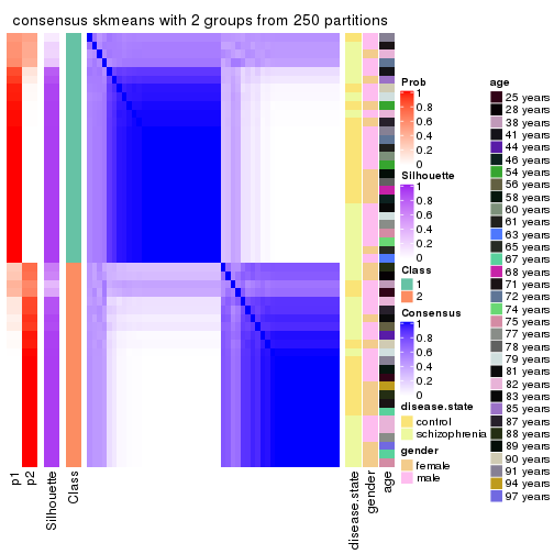
consensus_heatmap(res, k = 3)
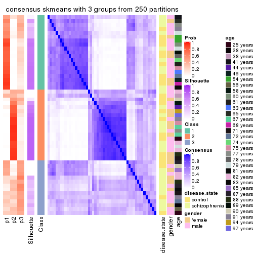
consensus_heatmap(res, k = 4)
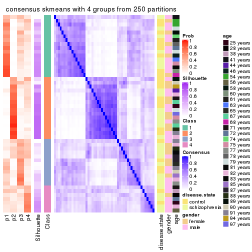
consensus_heatmap(res, k = 5)
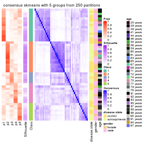
consensus_heatmap(res, k = 6)
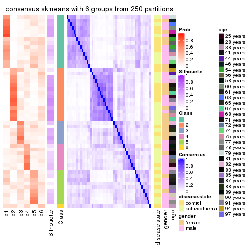
Heatmaps for the membership of samples in all partitions to see how consistent they are:
membership_heatmap(res, k = 2)
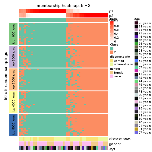
membership_heatmap(res, k = 3)
membership_heatmap(res, k = 4)
membership_heatmap(res, k = 5)
membership_heatmap(res, k = 6)
As soon as we have had the classes for columns, we can look for signatures which are significantly different between classes which can be candidate marks for certain classes. Following are the heatmaps for signatures.
Signature heatmaps where rows are scaled:
get_signatures(res, k = 2)
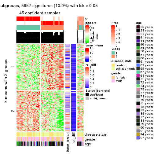
get_signatures(res, k = 3)
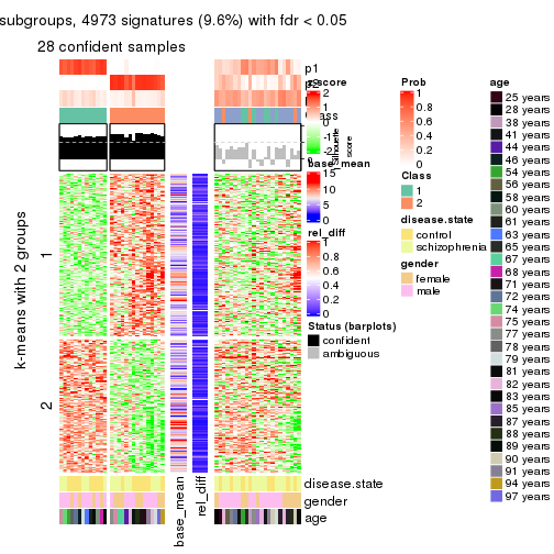
get_signatures(res, k = 4)
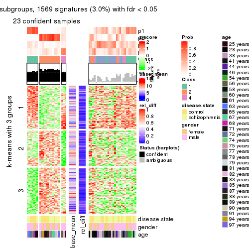
get_signatures(res, k = 5)
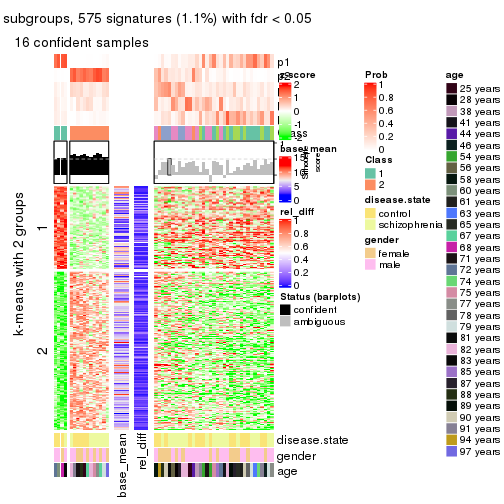
get_signatures(res, k = 6)

Signature heatmaps where rows are not scaled:
get_signatures(res, k = 2, scale_rows = FALSE)
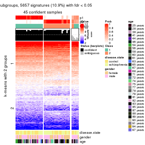
get_signatures(res, k = 3, scale_rows = FALSE)
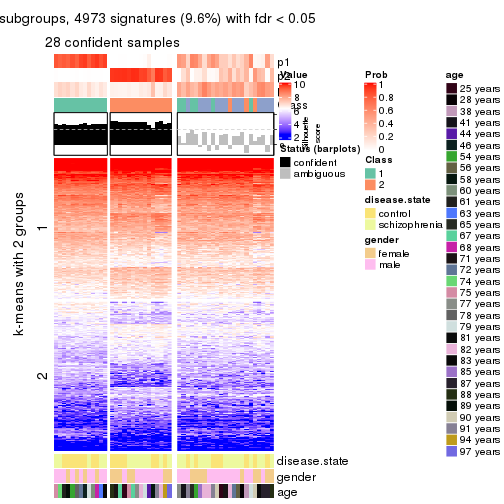
get_signatures(res, k = 4, scale_rows = FALSE)
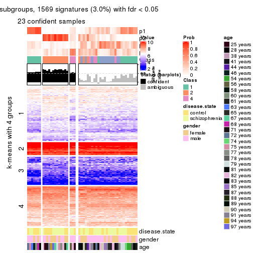
get_signatures(res, k = 5, scale_rows = FALSE)
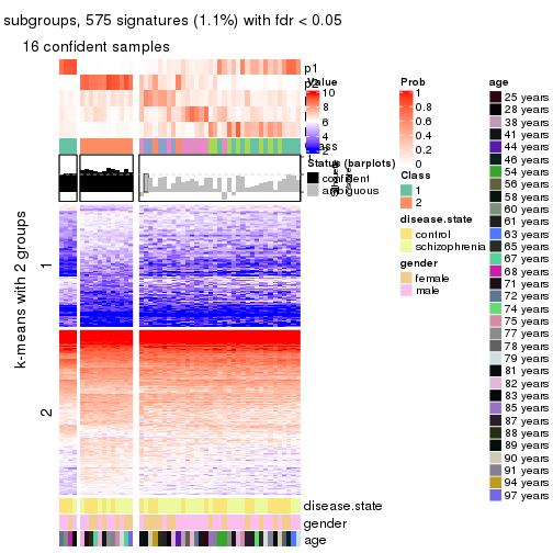
get_signatures(res, k = 6, scale_rows = FALSE)

Compare the overlap of signatures from different k:
compare_signatures(res)
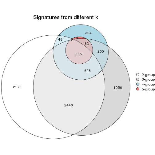
get_signature() returns a data frame invisibly. TO get the list of signatures, the function
call should be assigned to a variable explicitly. In following code, if plot argument is set
to FALSE, no heatmap is plotted while only the differential analysis is performed.
# code only for demonstration
tb = get_signature(res, k = ..., plot = FALSE)
An example of the output of tb is:
#>   which_row         fdr    mean_1    mean_2 scaled_mean_1 scaled_mean_2 km
#> 1        38 0.042760348  8.373488  9.131774    -0.5533452     0.5164555  1
#> 2        40 0.018707592  7.106213  8.469186    -0.6173731     0.5762149  1
#> 3        55 0.019134737 10.221463 11.207825    -0.6159697     0.5749050  1
#> 4        59 0.006059896  5.921854  7.869574    -0.6899429     0.6439467  1
#> 5        60 0.018055526  8.928898 10.211722    -0.6204761     0.5791110  1
#> 6        98 0.009384629 15.714769 14.887706     0.6635654    -0.6193277  2
...
The columns in tb are:
which_row: row indices corresponding to the input matrix.fdr: FDR for the differential test. mean_x: The mean value in group x.scaled_mean_x: The mean value in group x after rows are scaled.km: Row groups if k-means clustering is applied to rows.UMAP plot which shows how samples are separated.
dimension_reduction(res, k = 2, method = "UMAP")
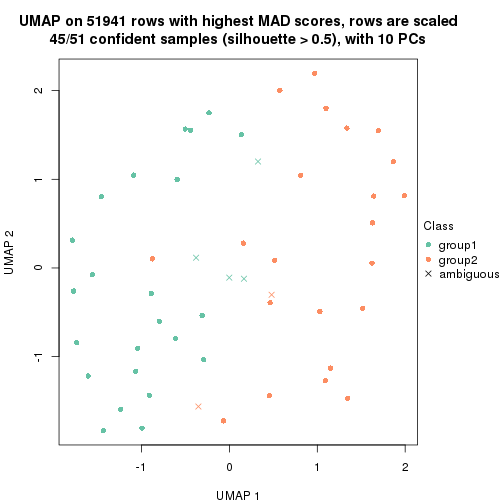
dimension_reduction(res, k = 3, method = "UMAP")
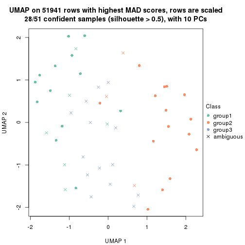
dimension_reduction(res, k = 4, method = "UMAP")
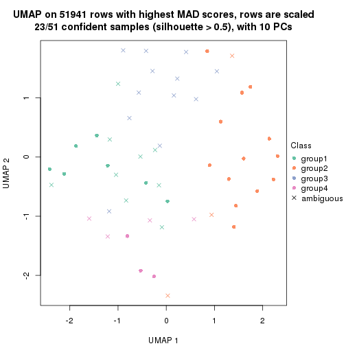
dimension_reduction(res, k = 5, method = "UMAP")
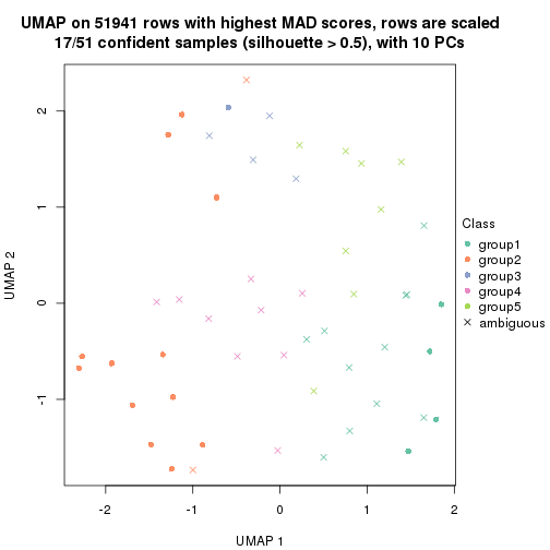
dimension_reduction(res, k = 6, method = "UMAP")
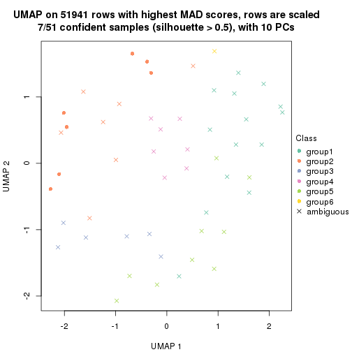
Following heatmap shows how subgroups are split when increasing k:
collect_classes(res)
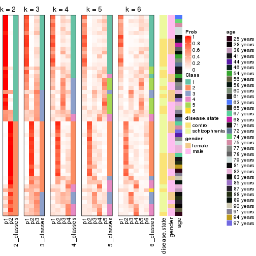
Test correlation between subgroups and known annotations. If the known annotation is numeric, one-way ANOVA test is applied, and if the known annotation is discrete, chi-squared contingency table test is applied.
test_to_known_factors(res)
#>              n disease.state(p) gender(p) age(p) k
#> MAD:skmeans 45            0.443     0.465  0.552 2
#> MAD:skmeans 28            0.684     0.638  0.405 3
#> MAD:skmeans 23            0.775     0.179  0.543 4
#> MAD:skmeans 17            0.319     0.378  0.201 5
#> MAD:skmeans  7               NA        NA     NA 6
If matrix rows can be associated to genes, consider to use functional_enrichment(res,
...) to perform function enrichment for the signature genes. See this vignette for more detailed explanations.
The object with results only for a single top-value method and a single partition method can be extracted as:
res = res_list["MAD", "pam"]
# you can also extract it by
# res = res_list["MAD:pam"]
A summary of res and all the functions that can be applied to it:
res
#> A 'ConsensusPartition' object with k = 2, 3, 4, 5, 6.
#>   On a matrix with 51941 rows and 51 columns.
#>   Top rows (1000, 2000, 3000, 4000, 5000) are extracted by 'MAD' method.
#>   Subgroups are detected by 'pam' method.
#>   Performed in total 1250 partitions by row resampling.
#>   Best k for subgroups seems to be 2.
#>
#> Following methods can be applied to this 'ConsensusPartition' object:
#>  [1] "cola_report"             "collect_classes"         "collect_plots"
#>  [4] "collect_stats"           "colnames"                "compare_signatures"
#>  [7] "consensus_heatmap"       "dimension_reduction"     "functional_enrichment"
#> [10] "get_anno_col"            "get_anno"                "get_classes"
#> [13] "get_consensus"           "get_matrix"              "get_membership"
#> [16] "get_param"               "get_signatures"          "get_stats"
#> [19] "is_best_k"               "is_stable_k"             "membership_heatmap"
#> [22] "ncol"                    "nrow"                    "plot_ecdf"
#> [25] "rownames"                "select_partition_number" "show"
#> [28] "suggest_best_k"          "test_to_known_factors"
collect_plots() function collects all the plots made from res for all k (number of partitions)
into one single page to provide an easy and fast comparison between different k.
collect_plots(res)
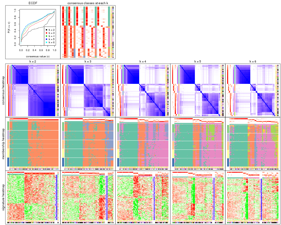
The plots are:
k and the heatmap of
predicted classes for each k.k.k.k.All the plots in panels can be made by individual functions and they are plotted later in this section.
select_partition_number() produces several plots showing different
statistics for choosing “optimized” k. There are following statistics:
k;k, the area increased is defined as \(A_k - A_{k-1}\).The detailed explanations of these statistics can be found in the cola vignette.
Generally speaking, lower PAC score, higher mean silhouette score or higher
concordance corresponds to better partition. Rand index and Jaccard index
measure how similar the current partition is compared to partition with k-1.
If they are too similar, we won't accept k is better than k-1.
select_partition_number(res)
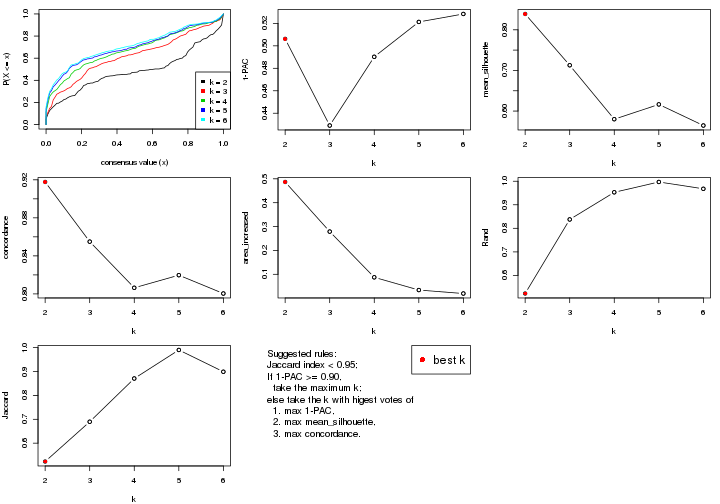
The numeric values for all these statistics can be obtained by get_stats().
get_stats(res)
#>   k 1-PAC mean_silhouette concordance area_increased  Rand Jaccard
#> 2 2 0.506           0.839       0.918         0.4868 0.523   0.523
#> 3 3 0.429           0.713       0.855         0.2790 0.838   0.690
#> 4 4 0.490           0.580       0.806         0.0874 0.953   0.871
#> 5 5 0.521           0.616       0.820         0.0341 0.997   0.990
#> 6 6 0.528           0.564       0.800         0.0196 0.968   0.899
suggest_best_k() suggests the best \(k\) based on these statistics. The rules are as follows:
suggest_best_k(res)
#> [1] 2
Following shows the table of the partitions (You need to click the show/hide
code output link to see it). The membership matrix (columns with name p*)
is inferred by
clue::cl_consensus()
function with the SE method. Basically the value in the membership matrix
represents the probability to belong to a certain group. The finall class
label for an item is determined with the group with highest probability it
belongs to.
In get_classes() function, the entropy is calculated from the membership
matrix and the silhouette score is calculated from the consensus matrix.
cbind(get_classes(res, k = 2), get_membership(res, k = 2))
#>           class entropy silhouette    p1    p2
#> GSM439800     2  0.6531     0.8276 0.168 0.832
#> GSM439790     2  0.0672     0.9012 0.008 0.992
#> GSM439827     2  0.0000     0.9005 0.000 1.000
#> GSM439811     2  0.2948     0.8957 0.052 0.948
#> GSM439795     2  0.2778     0.8956 0.048 0.952
#> GSM439805     2  0.4022     0.8850 0.080 0.920
#> GSM439781     2  0.6973     0.7820 0.188 0.812
#> GSM439807     1  0.1843     0.9032 0.972 0.028
#> GSM439820     2  0.0000     0.9005 0.000 1.000
#> GSM439784     1  0.1843     0.9051 0.972 0.028
#> GSM439824     2  0.4161     0.8834 0.084 0.916
#> GSM439794     2  0.7815     0.7510 0.232 0.768
#> GSM439809     1  0.0938     0.9115 0.988 0.012
#> GSM439785     2  0.0376     0.9010 0.004 0.996
#> GSM439803     2  0.2043     0.8988 0.032 0.968
#> GSM439778     1  0.8763     0.5854 0.704 0.296
#> GSM439791     1  0.0938     0.9116 0.988 0.012
#> GSM439786     2  0.4431     0.8764 0.092 0.908
#> GSM439828     2  0.0000     0.9005 0.000 1.000
#> GSM439806     1  0.7299     0.7311 0.796 0.204
#> GSM439815     2  0.6712     0.8197 0.176 0.824
#> GSM439817     2  0.5294     0.8564 0.120 0.880
#> GSM439796     2  0.0376     0.9010 0.004 0.996
#> GSM439798     2  0.5408     0.8498 0.124 0.876
#> GSM439821     2  0.0000     0.9005 0.000 1.000
#> GSM439823     2  0.0000     0.9005 0.000 1.000
#> GSM439813     1  0.0000     0.9127 1.000 0.000
#> GSM439801     2  0.0376     0.9010 0.004 0.996
#> GSM439810     2  0.7056     0.7815 0.192 0.808
#> GSM439783     1  0.0672     0.9122 0.992 0.008
#> GSM439826     2  0.0000     0.9005 0.000 1.000
#> GSM439812     1  0.0000     0.9127 1.000 0.000
#> GSM439818     2  0.6438     0.8190 0.164 0.836
#> GSM439792     1  0.0000     0.9127 1.000 0.000
#> GSM439802     1  0.0000     0.9127 1.000 0.000
#> GSM439825     2  0.0000     0.9005 0.000 1.000
#> GSM439780     1  0.0000     0.9127 1.000 0.000
#> GSM439787     2  0.9129     0.5286 0.328 0.672
#> GSM439808     2  0.8861     0.6237 0.304 0.696
#> GSM439804     2  0.6531     0.8143 0.168 0.832
#> GSM439822     2  0.7376     0.7667 0.208 0.792
#> GSM439816     1  0.8443     0.5838 0.728 0.272
#> GSM439789     1  0.0000     0.9127 1.000 0.000
#> GSM439799     2  0.0376     0.9010 0.004 0.996
#> GSM439814     1  0.0000     0.9127 1.000 0.000
#> GSM439782     1  0.9988     0.0742 0.520 0.480
#> GSM439779     1  0.0000     0.9127 1.000 0.000
#> GSM439793     1  0.2778     0.8921 0.952 0.048
#> GSM439788     1  0.1414     0.9092 0.980 0.020
#> GSM439797     2  0.0376     0.9010 0.004 0.996
#> GSM439819     2  0.0000     0.9005 0.000 1.000
cbind(get_classes(res, k = 3), get_membership(res, k = 3))
#>           class entropy silhouette    p1    p2    p3
#> GSM439800     2  0.4748     0.7414 0.144 0.832 0.024
#> GSM439790     2  0.1289     0.7882 0.032 0.968 0.000
#> GSM439827     3  0.4974     0.7133 0.000 0.236 0.764
#> GSM439811     3  0.4887     0.7159 0.000 0.228 0.772
#> GSM439795     2  0.3742     0.7667 0.036 0.892 0.072
#> GSM439805     2  0.3038     0.7788 0.104 0.896 0.000
#> GSM439781     2  0.6794     0.6195 0.196 0.728 0.076
#> GSM439807     1  0.2569     0.8722 0.936 0.032 0.032
#> GSM439820     2  0.3573     0.7373 0.004 0.876 0.120
#> GSM439784     1  0.1399     0.8929 0.968 0.028 0.004
#> GSM439824     2  0.6292     0.6007 0.044 0.740 0.216
#> GSM439794     2  0.5680     0.6557 0.212 0.764 0.024
#> GSM439809     1  0.0592     0.9008 0.988 0.012 0.000
#> GSM439785     2  0.0592     0.7838 0.012 0.988 0.000
#> GSM439803     2  0.1781     0.7855 0.020 0.960 0.020
#> GSM439778     1  0.5465     0.6144 0.712 0.288 0.000
#> GSM439791     1  0.0592     0.9009 0.988 0.012 0.000
#> GSM439786     2  0.3340     0.7634 0.120 0.880 0.000
#> GSM439828     3  0.6307     0.2768 0.000 0.488 0.512
#> GSM439806     1  0.5122     0.7245 0.788 0.200 0.012
#> GSM439815     2  0.4921     0.7237 0.164 0.816 0.020
#> GSM439817     2  0.6142     0.6224 0.040 0.748 0.212
#> GSM439796     2  0.1031     0.7778 0.000 0.976 0.024
#> GSM439798     2  0.4228     0.7302 0.148 0.844 0.008
#> GSM439821     3  0.5138     0.5756 0.000 0.252 0.748
#> GSM439823     2  0.3038     0.7508 0.000 0.896 0.104
#> GSM439813     1  0.0000     0.9017 1.000 0.000 0.000
#> GSM439801     2  0.1289     0.7882 0.032 0.968 0.000
#> GSM439810     2  0.4750     0.6448 0.216 0.784 0.000
#> GSM439783     1  0.0424     0.9017 0.992 0.008 0.000
#> GSM439826     2  0.5621     0.4305 0.000 0.692 0.308
#> GSM439812     1  0.0000     0.9017 1.000 0.000 0.000
#> GSM439818     2  0.7724     0.0102 0.052 0.552 0.396
#> GSM439792     1  0.0000     0.9017 1.000 0.000 0.000
#> GSM439802     1  0.0000     0.9017 1.000 0.000 0.000
#> GSM439825     3  0.2537     0.6932 0.000 0.080 0.920
#> GSM439780     1  0.0000     0.9017 1.000 0.000 0.000
#> GSM439787     3  0.9591     0.2921 0.232 0.296 0.472
#> GSM439808     3  0.5156     0.7114 0.008 0.216 0.776
#> GSM439804     2  0.4744     0.7314 0.136 0.836 0.028
#> GSM439822     3  0.7464     0.4387 0.040 0.400 0.560
#> GSM439816     1  0.6096     0.5379 0.704 0.280 0.016
#> GSM439789     1  0.0424     0.9003 0.992 0.000 0.008
#> GSM439799     2  0.1031     0.7777 0.000 0.976 0.024
#> GSM439814     1  0.0000     0.9017 1.000 0.000 0.000
#> GSM439782     1  0.6291     0.1428 0.532 0.468 0.000
#> GSM439779     1  0.0000     0.9017 1.000 0.000 0.000
#> GSM439793     1  0.1989     0.8799 0.948 0.048 0.004
#> GSM439788     1  0.0892     0.8986 0.980 0.020 0.000
#> GSM439797     2  0.1289     0.7882 0.032 0.968 0.000
#> GSM439819     3  0.1163     0.6556 0.000 0.028 0.972
cbind(get_classes(res, k = 4), get_membership(res, k = 4))
#>           class entropy silhouette    p1    p2    p3    p4
#> GSM439800     4  0.6098     0.4593 0.068 0.000 0.316 0.616
#> GSM439790     4  0.0336     0.6557 0.008 0.000 0.000 0.992
#> GSM439827     2  0.3172     0.6253 0.000 0.840 0.000 0.160
#> GSM439811     2  0.3024     0.6285 0.000 0.852 0.000 0.148
#> GSM439795     3  0.5353     0.1734 0.000 0.012 0.556 0.432
#> GSM439805     4  0.2197     0.6355 0.080 0.000 0.004 0.916
#> GSM439781     4  0.5240     0.4499 0.188 0.072 0.000 0.740
#> GSM439807     1  0.3725     0.7837 0.848 0.004 0.120 0.028
#> GSM439820     4  0.2859     0.6271 0.000 0.112 0.008 0.880
#> GSM439784     1  0.1151     0.8816 0.968 0.008 0.000 0.024
#> GSM439824     4  0.5196     0.5244 0.044 0.204 0.008 0.744
#> GSM439794     4  0.6991     0.3447 0.136 0.000 0.324 0.540
#> GSM439809     1  0.0469     0.8892 0.988 0.000 0.000 0.012
#> GSM439785     4  0.0188     0.6537 0.000 0.000 0.004 0.996
#> GSM439803     4  0.4086     0.6029 0.008 0.000 0.216 0.776
#> GSM439778     1  0.4431     0.5910 0.696 0.000 0.000 0.304
#> GSM439791     1  0.0469     0.8894 0.988 0.000 0.000 0.012
#> GSM439786     4  0.2281     0.6125 0.096 0.000 0.000 0.904
#> GSM439828     2  0.4981     0.0201 0.000 0.536 0.000 0.464
#> GSM439806     1  0.4011     0.7153 0.784 0.008 0.000 0.208
#> GSM439815     4  0.5783     0.5465 0.088 0.000 0.220 0.692
#> GSM439817     4  0.4970     0.5405 0.028 0.204 0.012 0.756
#> GSM439796     4  0.4564     0.5009 0.000 0.000 0.328 0.672
#> GSM439798     4  0.2814     0.5658 0.132 0.000 0.000 0.868
#> GSM439821     2  0.7576     0.0518 0.000 0.452 0.344 0.204
#> GSM439823     4  0.3182     0.6407 0.000 0.096 0.028 0.876
#> GSM439813     1  0.0000     0.8909 1.000 0.000 0.000 0.000
#> GSM439801     4  0.0927     0.6538 0.008 0.000 0.016 0.976
#> GSM439810     4  0.3710     0.4647 0.192 0.000 0.004 0.804
#> GSM439783     1  0.0336     0.8903 0.992 0.000 0.000 0.008
#> GSM439826     4  0.7113    -0.0153 0.000 0.132 0.384 0.484
#> GSM439812     1  0.0000     0.8909 1.000 0.000 0.000 0.000
#> GSM439818     3  0.7562     0.1124 0.016 0.136 0.508 0.340
#> GSM439792     1  0.0000     0.8909 1.000 0.000 0.000 0.000
#> GSM439802     1  0.0000     0.8909 1.000 0.000 0.000 0.000
#> GSM439825     2  0.2973     0.5614 0.000 0.884 0.096 0.020
#> GSM439780     1  0.0000     0.8909 1.000 0.000 0.000 0.000
#> GSM439787     3  0.8389    -0.1643 0.068 0.356 0.456 0.120
#> GSM439808     2  0.4036     0.6137 0.004 0.816 0.020 0.160
#> GSM439804     4  0.4957     0.4835 0.004 0.004 0.336 0.656
#> GSM439822     3  0.8154     0.1742 0.008 0.292 0.380 0.320
#> GSM439816     1  0.6650     0.3449 0.612 0.004 0.112 0.272
#> GSM439789     1  0.0188     0.8901 0.996 0.000 0.004 0.000
#> GSM439799     4  0.4343     0.5711 0.000 0.004 0.264 0.732
#> GSM439814     1  0.0000     0.8909 1.000 0.000 0.000 0.000
#> GSM439782     1  0.4998     0.1828 0.512 0.000 0.000 0.488
#> GSM439779     1  0.0000     0.8909 1.000 0.000 0.000 0.000
#> GSM439793     1  0.1576     0.8691 0.948 0.004 0.000 0.048
#> GSM439788     1  0.0817     0.8856 0.976 0.000 0.000 0.024
#> GSM439797     4  0.0469     0.6558 0.012 0.000 0.000 0.988
#> GSM439819     2  0.1211     0.5588 0.000 0.960 0.040 0.000
cbind(get_classes(res, k = 5), get_membership(res, k = 5))
#>           class entropy silhouette    p1    p2    p3    p4    p5
#> GSM439800     4  0.5979   0.490108 0.064 0.000 0.032 0.588 0.316
#> GSM439790     4  0.1408   0.702512 0.000 0.000 0.044 0.948 0.008
#> GSM439827     2  0.2583   0.628664 0.000 0.864 0.004 0.132 0.000
#> GSM439811     2  0.2536   0.629354 0.000 0.868 0.004 0.128 0.000
#> GSM439795     3  0.2171   0.656118 0.000 0.000 0.912 0.064 0.024
#> GSM439805     4  0.2293   0.686775 0.084 0.000 0.016 0.900 0.000
#> GSM439781     4  0.4571   0.536242 0.188 0.076 0.000 0.736 0.000
#> GSM439807     1  0.4326   0.754144 0.808 0.004 0.100 0.032 0.056
#> GSM439820     4  0.2959   0.680936 0.000 0.100 0.036 0.864 0.000
#> GSM439784     1  0.1106   0.875805 0.964 0.012 0.000 0.024 0.000
#> GSM439824     4  0.4484   0.623567 0.044 0.192 0.000 0.752 0.012
#> GSM439794     4  0.6124   0.392599 0.128 0.000 0.004 0.536 0.332
#> GSM439809     1  0.0566   0.883672 0.984 0.000 0.000 0.012 0.004
#> GSM439785     4  0.0162   0.700530 0.004 0.000 0.000 0.996 0.000
#> GSM439803     4  0.3643   0.650338 0.008 0.000 0.004 0.776 0.212
#> GSM439778     1  0.4681   0.612126 0.696 0.000 0.040 0.260 0.004
#> GSM439791     1  0.0566   0.883985 0.984 0.000 0.004 0.012 0.000
#> GSM439786     4  0.2700   0.673462 0.088 0.000 0.024 0.884 0.004
#> GSM439828     2  0.4256   0.094078 0.000 0.564 0.000 0.436 0.000
#> GSM439806     1  0.4195   0.714086 0.772 0.004 0.036 0.184 0.004
#> GSM439815     4  0.5582   0.608730 0.080 0.000 0.036 0.688 0.196
#> GSM439817     4  0.4363   0.618187 0.020 0.204 0.004 0.756 0.016
#> GSM439796     4  0.4118   0.529809 0.000 0.000 0.004 0.660 0.336
#> GSM439798     4  0.3257   0.634185 0.124 0.000 0.028 0.844 0.004
#> GSM439821     2  0.7874  -0.152972 0.000 0.432 0.292 0.124 0.152
#> GSM439823     4  0.2795   0.692054 0.000 0.100 0.000 0.872 0.028
#> GSM439813     1  0.0162   0.884522 0.996 0.000 0.000 0.000 0.004
#> GSM439801     4  0.1153   0.703251 0.008 0.000 0.024 0.964 0.004
#> GSM439810     4  0.3670   0.542804 0.188 0.000 0.012 0.792 0.008
#> GSM439783     1  0.0290   0.885123 0.992 0.000 0.000 0.008 0.000
#> GSM439826     4  0.6354  -0.066599 0.000 0.104 0.016 0.464 0.416
#> GSM439812     1  0.0324   0.884473 0.992 0.000 0.004 0.000 0.004
#> GSM439818     5  0.1911  -0.000775 0.000 0.036 0.028 0.004 0.932
#> GSM439792     1  0.0000   0.884098 1.000 0.000 0.000 0.000 0.000
#> GSM439802     1  0.0290   0.884658 0.992 0.000 0.008 0.000 0.000
#> GSM439825     2  0.3150   0.521502 0.000 0.864 0.024 0.016 0.096
#> GSM439780     1  0.0000   0.884098 1.000 0.000 0.000 0.000 0.000
#> GSM439787     3  0.5046   0.617139 0.036 0.216 0.716 0.028 0.004
#> GSM439808     2  0.4528   0.590948 0.000 0.752 0.104 0.144 0.000
#> GSM439804     4  0.4302   0.517911 0.004 0.000 0.004 0.648 0.344
#> GSM439822     5  0.7238   0.089864 0.004 0.248 0.016 0.324 0.408
#> GSM439816     1  0.6187   0.371523 0.600 0.000 0.032 0.272 0.096
#> GSM439789     1  0.0290   0.884099 0.992 0.000 0.000 0.000 0.008
#> GSM439799     4  0.3715   0.616439 0.000 0.000 0.004 0.736 0.260
#> GSM439814     1  0.0162   0.884522 0.996 0.000 0.000 0.000 0.004
#> GSM439782     1  0.4900   0.209174 0.512 0.000 0.024 0.464 0.000
#> GSM439779     1  0.0000   0.884098 1.000 0.000 0.000 0.000 0.000
#> GSM439793     1  0.1357   0.865308 0.948 0.004 0.000 0.048 0.000
#> GSM439788     1  0.0771   0.881359 0.976 0.000 0.004 0.020 0.000
#> GSM439797     4  0.0324   0.700285 0.004 0.000 0.004 0.992 0.000
#> GSM439819     2  0.1992   0.516281 0.000 0.924 0.044 0.000 0.032
cbind(get_classes(res, k = 6), get_membership(res, k = 6))
#> class entropy silhouette p1 p2 p3 p4 p5 p6
#> GSM439800 5 0.6717 0.25389 0.048 0.000 0.056 0.392 0.444 0.060
#> GSM439790 4 0.1845 0.62433 0.000 0.000 0.072 0.916 0.004 0.008
#> GSM439827 2 0.2178 0.58877 0.000 0.868 0.000 0.132 0.000 0.000
#> GSM439811 2 0.2135 0.58845 0.000 0.872 0.000 0.128 0.000 0.000
#> GSM439795 3 0.0692 0.57264 0.000 0.000 0.976 0.020 0.004 0.000
#> GSM439805 4 0.2265 0.60849 0.076 0.000 0.024 0.896 0.000 0.004
#> GSM439781 4 0.4054 0.42750 0.188 0.072 0.000 0.740 0.000 0.000
#> GSM439807 1 0.4369 0.74970 0.800 0.004 0.064 0.028 0.044 0.060
#> GSM439820 4 0.3006 0.60286 0.000 0.100 0.012 0.856 0.004 0.028
#> GSM439784 1 0.0993 0.87557 0.964 0.012 0.000 0.024 0.000 0.000
#> GSM439824 4 0.3854 0.52204 0.048 0.188 0.000 0.760 0.004 0.000
#> GSM439794 4 0.5913 0.00302 0.124 0.000 0.004 0.532 0.320 0.020
#> GSM439809 1 0.0508 0.88251 0.984 0.000 0.000 0.012 0.000 0.004
#> GSM439785 4 0.0436 0.63632 0.004 0.000 0.004 0.988 0.000 0.004
#> GSM439803 4 0.3541 0.51034 0.004 0.000 0.004 0.772 0.204 0.016
#> GSM439778 1 0.4651 0.60487 0.680 0.000 0.068 0.244 0.004 0.004
#> GSM439791 1 0.0622 0.88196 0.980 0.000 0.008 0.012 0.000 0.000
#> GSM439786 4 0.3516 0.57517 0.088 0.000 0.004 0.824 0.008 0.076
#> GSM439828 2 0.3823 -0.09587 0.000 0.564 0.000 0.436 0.000 0.000
#> GSM439806 1 0.4001 0.71929 0.768 0.004 0.052 0.168 0.000 0.008
#> GSM439815 4 0.5371 0.40719 0.068 0.000 0.036 0.680 0.196 0.020
#> GSM439817 4 0.3998 0.51098 0.024 0.204 0.004 0.752 0.016 0.000
#> GSM439796 4 0.4170 0.25857 0.000 0.000 0.004 0.648 0.328 0.020
#> GSM439798 4 0.3836 0.52808 0.124 0.000 0.008 0.788 0.000 0.080
#> GSM439821 2 0.8003 -0.07120 0.000 0.376 0.172 0.076 0.292 0.084
#> GSM439823 4 0.2558 0.61183 0.000 0.104 0.000 0.868 0.028 0.000
#> GSM439813 1 0.0291 0.88242 0.992 0.000 0.000 0.000 0.004 0.004
#> GSM439801 4 0.1180 0.63926 0.008 0.004 0.024 0.960 0.000 0.004
#> GSM439810 4 0.3733 0.40971 0.188 0.000 0.008 0.776 0.012 0.016
#> GSM439783 1 0.0260 0.88320 0.992 0.000 0.000 0.008 0.000 0.000
#> GSM439826 5 0.5489 0.52492 0.000 0.064 0.000 0.388 0.520 0.028
#> GSM439812 1 0.0363 0.88224 0.988 0.000 0.000 0.000 0.000 0.012
#> GSM439818 6 0.4059 0.00000 0.000 0.020 0.016 0.004 0.224 0.736
#> GSM439792 1 0.0000 0.88147 1.000 0.000 0.000 0.000 0.000 0.000
#> GSM439802 1 0.0862 0.87848 0.972 0.000 0.016 0.004 0.000 0.008
#> GSM439825 2 0.5009 0.30854 0.000 0.536 0.000 0.000 0.388 0.076
#> GSM439780 1 0.0000 0.88147 1.000 0.000 0.000 0.000 0.000 0.000
#> GSM439787 3 0.5558 0.58968 0.036 0.200 0.680 0.032 0.012 0.040
#> GSM439808 2 0.4566 0.54247 0.000 0.748 0.064 0.136 0.000 0.052
#> GSM439804 4 0.4410 0.24464 0.008 0.000 0.004 0.640 0.328 0.020
#> GSM439822 5 0.6265 0.46407 0.004 0.184 0.000 0.260 0.524 0.028
#> GSM439816 1 0.5866 0.31221 0.584 0.000 0.048 0.276 0.088 0.004
#> GSM439789 1 0.0260 0.88263 0.992 0.000 0.000 0.000 0.008 0.000
#> GSM439799 4 0.3767 0.42407 0.000 0.000 0.004 0.720 0.260 0.016
#> GSM439814 1 0.0291 0.88242 0.992 0.000 0.000 0.000 0.004 0.004
#> GSM439782 1 0.4847 0.20018 0.500 0.000 0.036 0.456 0.004 0.004
#> GSM439779 1 0.0000 0.88147 1.000 0.000 0.000 0.000 0.000 0.000
#> GSM439793 1 0.1219 0.86519 0.948 0.004 0.000 0.048 0.000 0.000
#> GSM439788 1 0.0632 0.88084 0.976 0.000 0.000 0.024 0.000 0.000
#> GSM439797 4 0.0436 0.63651 0.004 0.000 0.004 0.988 0.000 0.004
#> GSM439819 2 0.2854 0.43119 0.000 0.872 0.036 0.000 0.068 0.024
Heatmaps for the consensus matrix. It visualizes the probability of two samples to be in a same group.
consensus_heatmap(res, k = 2)
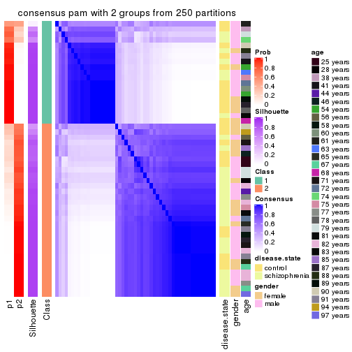
consensus_heatmap(res, k = 3)
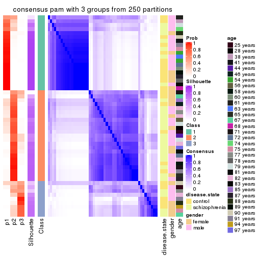
consensus_heatmap(res, k = 4)
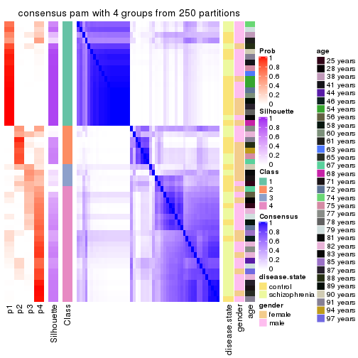
consensus_heatmap(res, k = 5)
consensus_heatmap(res, k = 6)
Heatmaps for the membership of samples in all partitions to see how consistent they are:
membership_heatmap(res, k = 2)
membership_heatmap(res, k = 3)
membership_heatmap(res, k = 4)
membership_heatmap(res, k = 5)
membership_heatmap(res, k = 6)
As soon as we have had the classes for columns, we can look for signatures which are significantly different between classes which can be candidate marks for certain classes. Following are the heatmaps for signatures.
Signature heatmaps where rows are scaled:
get_signatures(res, k = 2)
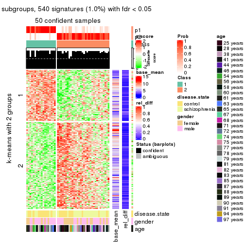
get_signatures(res, k = 3)
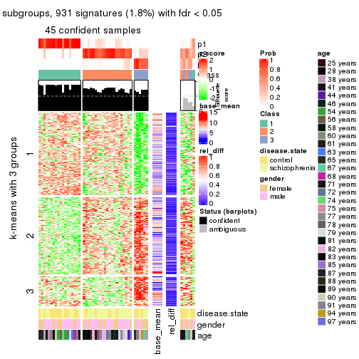
get_signatures(res, k = 4)
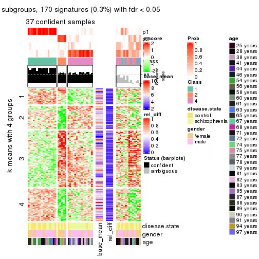
get_signatures(res, k = 5)
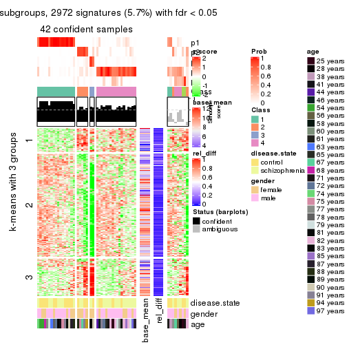
get_signatures(res, k = 6)
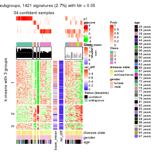
Signature heatmaps where rows are not scaled:
get_signatures(res, k = 2, scale_rows = FALSE)
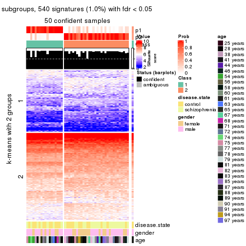
get_signatures(res, k = 3, scale_rows = FALSE)
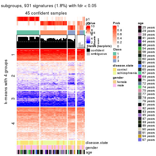
get_signatures(res, k = 4, scale_rows = FALSE)
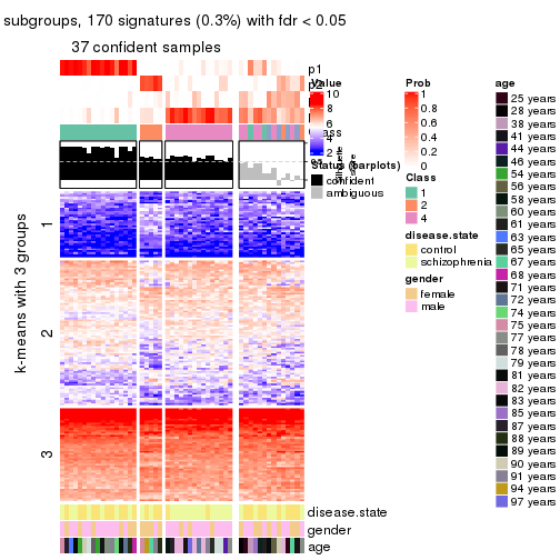
get_signatures(res, k = 5, scale_rows = FALSE)
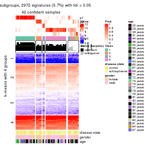
get_signatures(res, k = 6, scale_rows = FALSE)
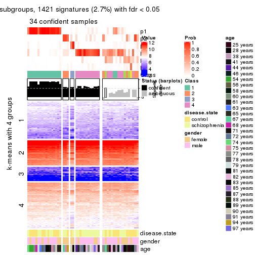
Compare the overlap of signatures from different k:
compare_signatures(res)
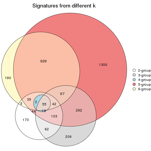
get_signature() returns a data frame invisibly. TO get the list of signatures, the function
call should be assigned to a variable explicitly. In following code, if plot argument is set
to FALSE, no heatmap is plotted while only the differential analysis is performed.
# code only for demonstration
tb = get_signature(res, k = ..., plot = FALSE)
An example of the output of tb is:
#> which_row fdr mean_1 mean_2 scaled_mean_1 scaled_mean_2 km
#> 1 38 0.042760348 8.373488 9.131774 -0.5533452 0.5164555 1
#> 2 40 0.018707592 7.106213 8.469186 -0.6173731 0.5762149 1
#> 3 55 0.019134737 10.221463 11.207825 -0.6159697 0.5749050 1
#> 4 59 0.006059896 5.921854 7.869574 -0.6899429 0.6439467 1
#> 5 60 0.018055526 8.928898 10.211722 -0.6204761 0.5791110 1
#> 6 98 0.009384629 15.714769 14.887706 0.6635654 -0.6193277 2
...
The columns in tb are:
which_row: row indices corresponding to the input matrix.fdr: FDR for the differential test. mean_x: The mean value in group x.scaled_mean_x: The mean value in group x after rows are scaled.km: Row groups if k-means clustering is applied to rows.UMAP plot which shows how samples are separated.
dimension_reduction(res, k = 2, method = "UMAP")
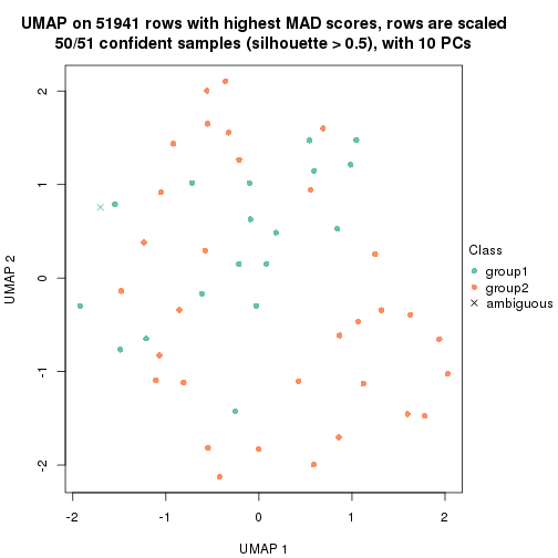
dimension_reduction(res, k = 3, method = "UMAP")
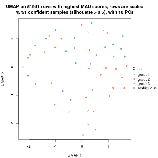
dimension_reduction(res, k = 4, method = "UMAP")
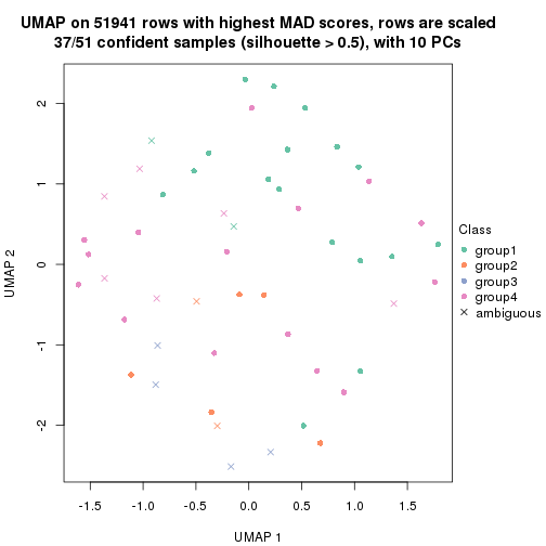
dimension_reduction(res, k = 5, method = "UMAP")
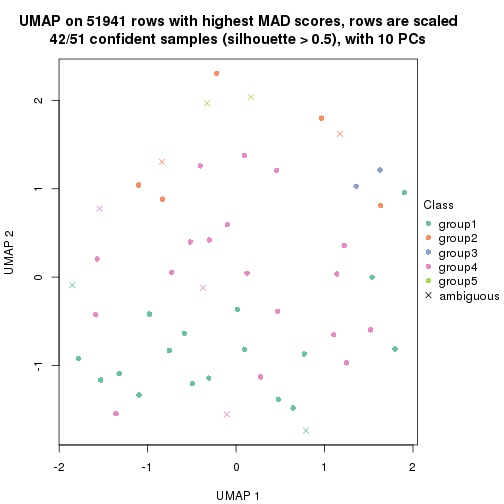
dimension_reduction(res, k = 6, method = "UMAP")
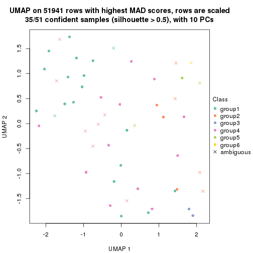
Following heatmap shows how subgroups are split when increasing k:
collect_classes(res)
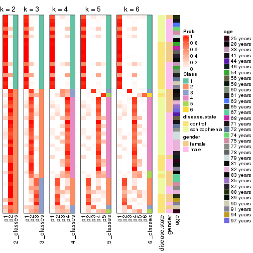
Test correlation between subgroups and known annotations. If the known annotation is numeric, one-way ANOVA test is applied, and if the known annotation is discrete, chi-squared contingency table test is applied.
test_to_known_factors(res)
#> n disease.state(p) gender(p) age(p) k
#> MAD:pam 50 0.1257 0.6738 0.353 2
#> MAD:pam 45 0.0243 0.2926 0.675 3
#> MAD:pam 37 0.0208 0.0517 0.446 4
#> MAD:pam 42 0.1362 0.0556 0.402 5
#> MAD:pam 35 0.0572 0.0411 0.651 6
If matrix rows can be associated to genes, consider to use functional_enrichment(res,
...) to perform function enrichment for the signature genes. See this vignette for more detailed explanations.
The object with results only for a single top-value method and a single partition method can be extracted as:
res = res_list["MAD", "mclust"]
# you can also extract it by
# res = res_list["MAD:mclust"]
A summary of res and all the functions that can be applied to it:
res
#> A 'ConsensusPartition' object with k = 2, 3, 4, 5, 6.
#> On a matrix with 51941 rows and 51 columns.
#> Top rows (1000, 2000, 3000, 4000, 5000) are extracted by 'MAD' method.
#> Subgroups are detected by 'mclust' method.
#> Performed in total 1250 partitions by row resampling.
#> Best k for subgroups seems to be 2.
#>
#> Following methods can be applied to this 'ConsensusPartition' object:
#> [1] "cola_report" "collect_classes" "collect_plots"
#> [4] "collect_stats" "colnames" "compare_signatures"
#> [7] "consensus_heatmap" "dimension_reduction" "functional_enrichment"
#> [10] "get_anno_col" "get_anno" "get_classes"
#> [13] "get_consensus" "get_matrix" "get_membership"
#> [16] "get_param" "get_signatures" "get_stats"
#> [19] "is_best_k" "is_stable_k" "membership_heatmap"
#> [22] "ncol" "nrow" "plot_ecdf"
#> [25] "rownames" "select_partition_number" "show"
#> [28] "suggest_best_k" "test_to_known_factors"
collect_plots() function collects all the plots made from res for all k (number of partitions)
into one single page to provide an easy and fast comparison between different k.
collect_plots(res)
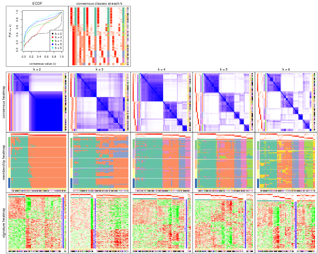
The plots are:
k and the heatmap of
predicted classes for each k.k.k.k.All the plots in panels can be made by individual functions and they are plotted later in this section.
select_partition_number() produces several plots showing different
statistics for choosing “optimized” k. There are following statistics:
k;k, the area increased is defined as \(A_k - A_{k-1}\).The detailed explanations of these statistics can be found in the cola vignette.
Generally speaking, lower PAC score, higher mean silhouette score or higher
concordance corresponds to better partition. Rand index and Jaccard index
measure how similar the current partition is compared to partition with k-1.
If they are too similar, we won't accept k is better than k-1.
select_partition_number(res)
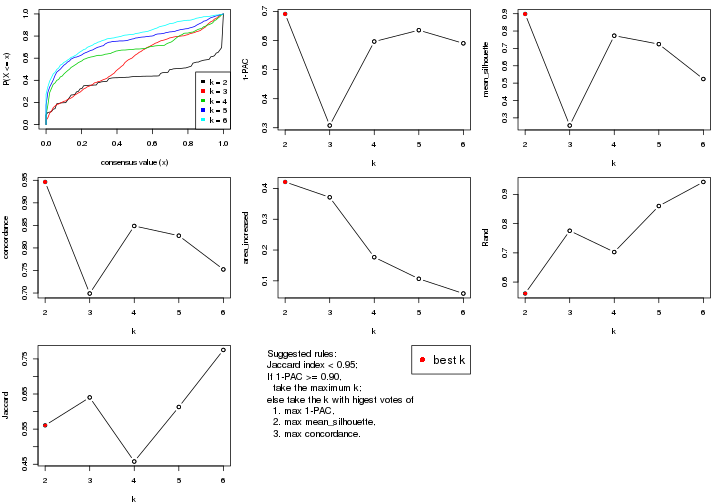
The numeric values for all these statistics can be obtained by get_stats().
get_stats(res)
#> k 1-PAC mean_silhouette concordance area_increased Rand Jaccard
#> 2 2 0.691 0.898 0.946 0.4211 0.561 0.561
#> 3 3 0.308 0.256 0.699 0.3713 0.776 0.640
#> 4 4 0.597 0.773 0.849 0.1767 0.703 0.458
#> 5 5 0.636 0.725 0.827 0.1067 0.860 0.613
#> 6 6 0.590 0.524 0.752 0.0588 0.943 0.775
suggest_best_k() suggests the best \(k\) based on these statistics. The rules are as follows:
suggest_best_k(res)
#> [1] 2
Following shows the table of the partitions (You need to click the show/hide
code output link to see it). The membership matrix (columns with name p*)
is inferred by
clue::cl_consensus()
function with the SE method. Basically the value in the membership matrix
represents the probability to belong to a certain group. The finall class
label for an item is determined with the group with highest probability it
belongs to.
In get_classes() function, the entropy is calculated from the membership
matrix and the silhouette score is calculated from the consensus matrix.
cbind(get_classes(res, k = 2), get_membership(res, k = 2))
#> class entropy silhouette p1 p2
#> GSM439800 2 0.0000 0.965 0.000 1.000
#> GSM439790 1 0.5178 0.882 0.884 0.116
#> GSM439827 2 0.0000 0.965 0.000 1.000
#> GSM439811 2 0.0000 0.965 0.000 1.000
#> GSM439795 2 0.0000 0.965 0.000 1.000
#> GSM439805 2 0.0000 0.965 0.000 1.000
#> GSM439781 2 0.4022 0.889 0.080 0.920
#> GSM439807 2 0.0000 0.965 0.000 1.000
#> GSM439820 2 0.0000 0.965 0.000 1.000
#> GSM439784 2 0.1184 0.953 0.016 0.984
#> GSM439824 2 0.0000 0.965 0.000 1.000
#> GSM439794 2 0.0000 0.965 0.000 1.000
#> GSM439809 1 0.0672 0.885 0.992 0.008
#> GSM439785 2 0.2778 0.924 0.048 0.952
#> GSM439803 2 0.0000 0.965 0.000 1.000
#> GSM439778 1 0.3114 0.892 0.944 0.056
#> GSM439791 1 0.0000 0.882 1.000 0.000
#> GSM439786 2 0.8955 0.470 0.312 0.688
#> GSM439828 2 0.0000 0.965 0.000 1.000
#> GSM439806 1 0.7453 0.811 0.788 0.212
#> GSM439815 1 0.9286 0.612 0.656 0.344
#> GSM439817 2 0.0000 0.965 0.000 1.000
#> GSM439796 2 0.0000 0.965 0.000 1.000
#> GSM439798 2 0.0000 0.965 0.000 1.000
#> GSM439821 2 0.0000 0.965 0.000 1.000
#> GSM439823 2 0.0000 0.965 0.000 1.000
#> GSM439813 1 0.2043 0.890 0.968 0.032
#> GSM439801 2 0.0000 0.965 0.000 1.000
#> GSM439810 1 0.5737 0.868 0.864 0.136
#> GSM439783 1 0.5519 0.879 0.872 0.128
#> GSM439826 2 0.0000 0.965 0.000 1.000
#> GSM439812 1 0.0000 0.882 1.000 0.000
#> GSM439818 2 0.0000 0.965 0.000 1.000
#> GSM439792 1 0.0000 0.882 1.000 0.000
#> GSM439802 2 0.0000 0.965 0.000 1.000
#> GSM439825 2 0.0000 0.965 0.000 1.000
#> GSM439780 1 0.6438 0.857 0.836 0.164
#> GSM439787 2 0.0000 0.965 0.000 1.000
#> GSM439808 2 0.0000 0.965 0.000 1.000
#> GSM439804 2 0.0000 0.965 0.000 1.000
#> GSM439822 2 0.0000 0.965 0.000 1.000
#> GSM439816 2 0.0000 0.965 0.000 1.000
#> GSM439789 2 0.9393 0.339 0.356 0.644
#> GSM439799 2 0.0000 0.965 0.000 1.000
#> GSM439814 1 0.2948 0.892 0.948 0.052
#> GSM439782 1 0.6887 0.827 0.816 0.184
#> GSM439779 1 0.0000 0.882 1.000 0.000
#> GSM439793 2 0.6801 0.749 0.180 0.820
#> GSM439788 1 0.8661 0.704 0.712 0.288
#> GSM439797 2 0.1843 0.943 0.028 0.972
#> GSM439819 2 0.0000 0.965 0.000 1.000
cbind(get_classes(res, k = 3), get_membership(res, k = 3))
#> class entropy silhouette p1 p2 p3
#> GSM439800 2 0.6850 0.3125 0.120 0.740 0.140
#> GSM439790 1 0.2680 0.8468 0.924 0.068 0.008
#> GSM439827 2 0.6305 -0.7590 0.000 0.516 0.484
#> GSM439811 2 0.6305 -0.7590 0.000 0.516 0.484
#> GSM439795 2 0.2636 0.2609 0.020 0.932 0.048
#> GSM439805 2 0.5093 0.3151 0.088 0.836 0.076
#> GSM439781 1 0.9431 0.4566 0.500 0.280 0.220
#> GSM439807 2 0.5939 0.3381 0.140 0.788 0.072
#> GSM439820 2 0.6442 -0.7198 0.004 0.564 0.432
#> GSM439784 2 0.7130 0.1580 0.432 0.544 0.024
#> GSM439824 2 0.6779 -0.7819 0.012 0.544 0.444
#> GSM439794 2 0.8206 0.3344 0.196 0.640 0.164
#> GSM439809 1 0.1919 0.8451 0.956 0.020 0.024
#> GSM439785 2 0.6192 0.2065 0.420 0.580 0.000
#> GSM439803 2 0.8878 0.3281 0.216 0.576 0.208
#> GSM439778 1 0.1950 0.8472 0.952 0.040 0.008
#> GSM439791 1 0.0592 0.8346 0.988 0.000 0.012
#> GSM439786 1 0.8879 0.5827 0.576 0.212 0.212
#> GSM439828 2 0.6280 -0.7553 0.000 0.540 0.460
#> GSM439806 1 0.4094 0.8296 0.872 0.100 0.028
#> GSM439815 1 0.4700 0.7735 0.812 0.180 0.008
#> GSM439817 2 0.6783 -0.6672 0.016 0.588 0.396
#> GSM439796 2 0.8562 0.3168 0.184 0.608 0.208
#> GSM439798 1 0.9653 0.3260 0.448 0.328 0.224
#> GSM439821 2 0.6252 -0.7605 0.000 0.556 0.444
#> GSM439823 2 0.6215 -0.7670 0.000 0.572 0.428
#> GSM439813 1 0.1289 0.8470 0.968 0.032 0.000
#> GSM439801 2 0.2947 0.2607 0.020 0.920 0.060
#> GSM439810 1 0.1877 0.8434 0.956 0.032 0.012
#> GSM439783 1 0.2866 0.8437 0.916 0.076 0.008
#> GSM439826 3 0.6309 0.9864 0.000 0.496 0.504
#> GSM439812 1 0.0592 0.8346 0.988 0.000 0.012
#> GSM439818 2 0.6308 -0.9492 0.000 0.508 0.492
#> GSM439792 1 0.1315 0.8407 0.972 0.008 0.020
#> GSM439802 2 0.7384 0.3020 0.272 0.660 0.068
#> GSM439825 2 0.6308 -0.9423 0.000 0.508 0.492
#> GSM439780 1 0.2866 0.8451 0.916 0.076 0.008
#> GSM439787 2 0.3550 0.2157 0.024 0.896 0.080
#> GSM439808 2 0.6282 -0.4759 0.012 0.664 0.324
#> GSM439804 2 0.8689 0.3260 0.204 0.596 0.200
#> GSM439822 3 0.6308 0.9864 0.000 0.492 0.508
#> GSM439816 2 0.6999 0.3193 0.268 0.680 0.052
#> GSM439789 1 0.5171 0.7293 0.784 0.204 0.012
#> GSM439799 2 0.3482 -0.0387 0.000 0.872 0.128
#> GSM439814 1 0.1482 0.8450 0.968 0.020 0.012
#> GSM439782 1 0.2680 0.8462 0.924 0.068 0.008
#> GSM439779 1 0.0592 0.8346 0.988 0.000 0.012
#> GSM439793 1 0.9148 0.5430 0.544 0.236 0.220
#> GSM439788 1 0.7199 0.7328 0.704 0.092 0.204
#> GSM439797 2 0.6600 0.2879 0.384 0.604 0.012
#> GSM439819 2 0.6267 -0.7534 0.000 0.548 0.452
cbind(get_classes(res, k = 4), get_membership(res, k = 4))
#> class entropy silhouette p1 p2 p3 p4
#> GSM439800 4 0.5760 0.860 0.004 0.140 0.132 0.724
#> GSM439790 1 0.1486 0.859 0.960 0.008 0.024 0.008
#> GSM439827 2 0.2611 0.760 0.000 0.896 0.008 0.096
#> GSM439811 2 0.2611 0.760 0.000 0.896 0.008 0.096
#> GSM439795 3 0.3048 0.851 0.000 0.108 0.876 0.016
#> GSM439805 3 0.2674 0.861 0.004 0.068 0.908 0.020
#> GSM439781 1 0.5366 0.695 0.696 0.008 0.268 0.028
#> GSM439807 3 0.2911 0.861 0.016 0.072 0.900 0.012
#> GSM439820 2 0.0921 0.818 0.000 0.972 0.028 0.000
#> GSM439784 1 0.6363 0.639 0.672 0.200 0.120 0.008
#> GSM439824 2 0.3441 0.780 0.004 0.840 0.004 0.152
#> GSM439794 4 0.4238 0.950 0.004 0.108 0.060 0.828
#> GSM439809 1 0.0712 0.859 0.984 0.004 0.008 0.004
#> GSM439785 1 0.5968 0.713 0.736 0.136 0.100 0.028
#> GSM439803 4 0.4368 0.947 0.016 0.096 0.056 0.832
#> GSM439778 1 0.0992 0.859 0.976 0.004 0.012 0.008
#> GSM439791 1 0.0336 0.857 0.992 0.000 0.008 0.000
#> GSM439786 1 0.4993 0.712 0.728 0.020 0.244 0.008
#> GSM439828 2 0.0804 0.818 0.000 0.980 0.008 0.012
#> GSM439806 1 0.2099 0.855 0.936 0.040 0.020 0.004
#> GSM439815 1 0.2821 0.851 0.912 0.028 0.040 0.020
#> GSM439817 2 0.1356 0.819 0.000 0.960 0.032 0.008
#> GSM439796 4 0.4041 0.949 0.004 0.100 0.056 0.840
#> GSM439798 1 0.6060 0.447 0.572 0.028 0.388 0.012
#> GSM439821 2 0.2021 0.823 0.000 0.936 0.024 0.040
#> GSM439823 2 0.2335 0.821 0.000 0.920 0.020 0.060
#> GSM439813 1 0.0524 0.858 0.988 0.000 0.008 0.004
#> GSM439801 3 0.2593 0.861 0.000 0.080 0.904 0.016
#> GSM439810 1 0.0992 0.860 0.976 0.012 0.008 0.004
#> GSM439783 1 0.1854 0.858 0.948 0.020 0.008 0.024
#> GSM439826 2 0.3945 0.753 0.000 0.780 0.004 0.216
#> GSM439812 1 0.0524 0.856 0.988 0.000 0.008 0.004
#> GSM439818 2 0.4576 0.695 0.000 0.728 0.012 0.260
#> GSM439792 1 0.0469 0.858 0.988 0.000 0.012 0.000
#> GSM439802 3 0.5433 0.614 0.220 0.056 0.720 0.004
#> GSM439825 2 0.3591 0.785 0.000 0.824 0.008 0.168
#> GSM439780 1 0.1739 0.859 0.952 0.016 0.024 0.008
#> GSM439787 3 0.3893 0.772 0.000 0.196 0.796 0.008
#> GSM439808 2 0.4454 0.502 0.000 0.692 0.308 0.000
#> GSM439804 4 0.4372 0.949 0.012 0.104 0.056 0.828
#> GSM439822 2 0.3908 0.756 0.000 0.784 0.004 0.212
#> GSM439816 1 0.9218 -0.105 0.372 0.324 0.088 0.216
#> GSM439789 1 0.3229 0.818 0.880 0.072 0.000 0.048
#> GSM439799 2 0.7304 0.215 0.000 0.492 0.164 0.344
#> GSM439814 1 0.0859 0.859 0.980 0.008 0.008 0.004
#> GSM439782 1 0.1377 0.860 0.964 0.008 0.020 0.008
#> GSM439779 1 0.0336 0.857 0.992 0.000 0.008 0.000
#> GSM439793 1 0.5060 0.737 0.736 0.008 0.228 0.028
#> GSM439788 1 0.3824 0.818 0.844 0.008 0.124 0.024
#> GSM439797 1 0.6246 0.696 0.712 0.136 0.128 0.024
#> GSM439819 2 0.1833 0.822 0.000 0.944 0.024 0.032
cbind(get_classes(res, k = 5), get_membership(res, k = 5))
#> class entropy silhouette p1 p2 p3 p4 p5
#> GSM439800 4 0.5224 0.6688 0.000 0.140 0.176 0.684 0.000
#> GSM439790 1 0.3508 0.7742 0.832 0.004 0.028 0.004 0.132
#> GSM439827 2 0.2173 0.7208 0.000 0.920 0.012 0.052 0.016
#> GSM439811 2 0.2374 0.7214 0.000 0.912 0.020 0.052 0.016
#> GSM439795 3 0.1638 0.8568 0.000 0.064 0.932 0.004 0.000
#> GSM439805 3 0.2407 0.8580 0.008 0.036 0.916 0.008 0.032
#> GSM439781 5 0.3376 0.8184 0.128 0.004 0.024 0.004 0.840
#> GSM439807 3 0.2108 0.8642 0.004 0.036 0.928 0.008 0.024
#> GSM439820 2 0.1357 0.7528 0.000 0.948 0.048 0.000 0.004
#> GSM439784 5 0.7002 0.3205 0.136 0.340 0.028 0.008 0.488
#> GSM439824 2 0.4413 0.6807 0.004 0.740 0.004 0.220 0.032
#> GSM439794 4 0.2104 0.9032 0.000 0.060 0.024 0.916 0.000
#> GSM439809 1 0.1908 0.8326 0.908 0.000 0.000 0.000 0.092
#> GSM439785 1 0.8004 0.0861 0.472 0.272 0.048 0.044 0.164
#> GSM439803 4 0.2321 0.8972 0.024 0.044 0.016 0.916 0.000
#> GSM439778 1 0.2060 0.8565 0.928 0.000 0.036 0.024 0.012
#> GSM439791 1 0.0703 0.8625 0.976 0.000 0.000 0.000 0.024
#> GSM439786 5 0.4513 0.7936 0.192 0.008 0.052 0.000 0.748
#> GSM439828 2 0.0451 0.7504 0.000 0.988 0.004 0.008 0.000
#> GSM439806 1 0.4491 0.3123 0.624 0.004 0.008 0.000 0.364
#> GSM439815 1 0.3615 0.8276 0.864 0.024 0.048 0.032 0.032
#> GSM439817 2 0.2277 0.7540 0.000 0.916 0.052 0.016 0.016
#> GSM439796 4 0.1626 0.9088 0.000 0.044 0.016 0.940 0.000
#> GSM439798 5 0.3788 0.7793 0.104 0.004 0.072 0.000 0.820
#> GSM439821 2 0.2331 0.7568 0.000 0.908 0.024 0.004 0.064
#> GSM439823 2 0.2956 0.7563 0.000 0.884 0.020 0.060 0.036
#> GSM439813 1 0.1617 0.8640 0.948 0.000 0.020 0.012 0.020
#> GSM439801 3 0.1282 0.8623 0.000 0.044 0.952 0.004 0.000
#> GSM439810 1 0.0510 0.8625 0.984 0.000 0.000 0.000 0.016
#> GSM439783 1 0.3124 0.8294 0.884 0.028 0.016 0.056 0.016
#> GSM439826 2 0.5010 0.6637 0.000 0.688 0.000 0.224 0.088
#> GSM439812 1 0.0609 0.8625 0.980 0.000 0.000 0.000 0.020
#> GSM439818 2 0.5137 0.6512 0.000 0.676 0.004 0.244 0.076
#> GSM439792 1 0.1792 0.8386 0.916 0.000 0.000 0.000 0.084
#> GSM439802 3 0.4357 0.7449 0.088 0.032 0.808 0.004 0.068
#> GSM439825 2 0.4696 0.7024 0.000 0.740 0.004 0.172 0.084
#> GSM439780 1 0.2654 0.8510 0.900 0.000 0.040 0.016 0.044
#> GSM439787 3 0.4421 0.5901 0.000 0.268 0.704 0.004 0.024
#> GSM439808 2 0.3074 0.6719 0.000 0.804 0.196 0.000 0.000
#> GSM439804 4 0.1913 0.9094 0.008 0.044 0.016 0.932 0.000
#> GSM439822 2 0.5185 0.6634 0.000 0.684 0.004 0.220 0.092
#> GSM439816 2 0.7040 0.3491 0.124 0.504 0.032 0.328 0.012
#> GSM439789 1 0.3332 0.8077 0.868 0.048 0.012 0.064 0.008
#> GSM439799 2 0.6786 0.4067 0.000 0.532 0.296 0.132 0.040
#> GSM439814 1 0.0404 0.8627 0.988 0.000 0.000 0.000 0.012
#> GSM439782 1 0.2165 0.8553 0.924 0.000 0.036 0.024 0.016
#> GSM439779 1 0.0404 0.8629 0.988 0.000 0.000 0.000 0.012
#> GSM439793 5 0.3169 0.8241 0.140 0.004 0.016 0.000 0.840
#> GSM439788 5 0.3976 0.7858 0.216 0.004 0.020 0.000 0.760
#> GSM439797 2 0.8456 -0.2354 0.312 0.328 0.060 0.032 0.268
#> GSM439819 2 0.1310 0.7568 0.000 0.956 0.020 0.000 0.024
cbind(get_classes(res, k = 6), get_membership(res, k = 6))
#> class entropy silhouette p1 p2 p3 p4 p5 p6
#> GSM439800 4 0.3521 0.7656 0.000 0.120 0.060 0.812 0.000 0.008
#> GSM439790 1 0.4828 0.5735 0.668 0.000 0.004 0.000 0.220 0.108
#> GSM439827 2 0.3169 0.3956 0.000 0.852 0.020 0.024 0.008 0.096
#> GSM439811 2 0.3169 0.3956 0.000 0.852 0.020 0.024 0.008 0.096
#> GSM439795 3 0.2194 0.8187 0.000 0.040 0.912 0.036 0.004 0.008
#> GSM439805 3 0.1801 0.8231 0.000 0.004 0.924 0.016 0.056 0.000
#> GSM439781 5 0.2485 0.7218 0.084 0.008 0.024 0.000 0.884 0.000
#> GSM439807 3 0.1483 0.8335 0.000 0.012 0.944 0.008 0.036 0.000
#> GSM439820 2 0.2265 0.4399 0.000 0.900 0.068 0.008 0.000 0.024
#> GSM439784 5 0.5416 0.5373 0.112 0.228 0.020 0.004 0.636 0.000
#> GSM439824 2 0.5618 -0.1020 0.000 0.624 0.032 0.148 0.000 0.196
#> GSM439794 4 0.1442 0.9257 0.000 0.040 0.012 0.944 0.004 0.000
#> GSM439809 1 0.2768 0.6705 0.832 0.000 0.000 0.000 0.156 0.012
#> GSM439785 1 0.8009 -0.1113 0.336 0.256 0.052 0.060 0.288 0.008
#> GSM439803 4 0.1096 0.9332 0.000 0.020 0.008 0.964 0.004 0.004
#> GSM439778 1 0.3898 0.6701 0.684 0.000 0.000 0.000 0.020 0.296
#> GSM439791 1 0.1757 0.7302 0.916 0.000 0.000 0.000 0.076 0.008
#> GSM439786 5 0.3290 0.7043 0.132 0.004 0.044 0.000 0.820 0.000
#> GSM439828 2 0.1218 0.4293 0.000 0.956 0.004 0.012 0.000 0.028
#> GSM439806 5 0.4442 0.1198 0.476 0.004 0.004 0.000 0.504 0.012
#> GSM439815 1 0.6683 0.6125 0.600 0.016 0.028 0.068 0.096 0.192
#> GSM439817 2 0.3243 0.3887 0.000 0.844 0.064 0.016 0.000 0.076
#> GSM439796 4 0.0806 0.9365 0.000 0.020 0.008 0.972 0.000 0.000
#> GSM439798 5 0.2631 0.7001 0.068 0.008 0.044 0.000 0.880 0.000
#> GSM439821 2 0.4346 0.0368 0.000 0.676 0.020 0.020 0.000 0.284
#> GSM439823 2 0.4120 0.2653 0.000 0.780 0.024 0.056 0.004 0.136
#> GSM439813 1 0.2930 0.7395 0.840 0.000 0.000 0.000 0.036 0.124
#> GSM439801 3 0.0964 0.8296 0.000 0.016 0.968 0.012 0.004 0.000
#> GSM439810 1 0.1049 0.7410 0.960 0.000 0.000 0.000 0.032 0.008
#> GSM439783 1 0.5067 0.6939 0.756 0.028 0.012 0.048 0.084 0.072
#> GSM439826 6 0.5669 0.9775 0.000 0.412 0.008 0.104 0.004 0.472
#> GSM439812 1 0.0972 0.7397 0.964 0.000 0.000 0.000 0.028 0.008
#> GSM439818 2 0.5871 -0.7265 0.000 0.416 0.004 0.168 0.000 0.412
#> GSM439792 1 0.2980 0.6420 0.808 0.000 0.000 0.000 0.180 0.012
#> GSM439802 3 0.5588 0.5554 0.156 0.012 0.672 0.008 0.128 0.024
#> GSM439825 2 0.5225 -0.6168 0.000 0.496 0.004 0.080 0.000 0.420
#> GSM439780 1 0.4341 0.6584 0.668 0.000 0.008 0.000 0.032 0.292
#> GSM439787 3 0.3828 0.5324 0.000 0.252 0.724 0.000 0.016 0.008
#> GSM439808 2 0.3878 0.3565 0.000 0.736 0.228 0.004 0.000 0.032
#> GSM439804 4 0.0806 0.9365 0.000 0.020 0.008 0.972 0.000 0.000
#> GSM439822 6 0.5571 0.9776 0.000 0.412 0.004 0.104 0.004 0.476
#> GSM439816 2 0.8217 -0.0981 0.168 0.372 0.036 0.312 0.048 0.064
#> GSM439789 1 0.5093 0.6668 0.752 0.052 0.004 0.080 0.068 0.044
#> GSM439799 2 0.7427 -0.2127 0.000 0.400 0.188 0.220 0.000 0.192
#> GSM439814 1 0.1124 0.7413 0.956 0.000 0.000 0.000 0.036 0.008
#> GSM439782 1 0.3993 0.6659 0.676 0.000 0.000 0.000 0.024 0.300
#> GSM439779 1 0.2106 0.7285 0.904 0.000 0.000 0.000 0.064 0.032
#> GSM439793 5 0.2113 0.7262 0.092 0.004 0.008 0.000 0.896 0.000
#> GSM439788 5 0.2841 0.7034 0.164 0.000 0.012 0.000 0.824 0.000
#> GSM439797 5 0.7824 0.1440 0.188 0.284 0.076 0.048 0.400 0.004
#> GSM439819 2 0.2844 0.3950 0.000 0.860 0.020 0.016 0.000 0.104
Heatmaps for the consensus matrix. It visualizes the probability of two samples to be in a same group.
consensus_heatmap(res, k = 2)
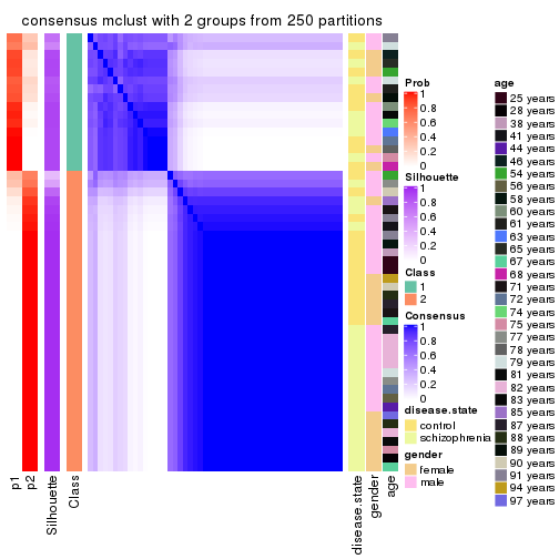
consensus_heatmap(res, k = 3)
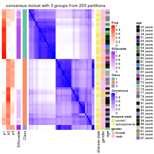
consensus_heatmap(res, k = 4)
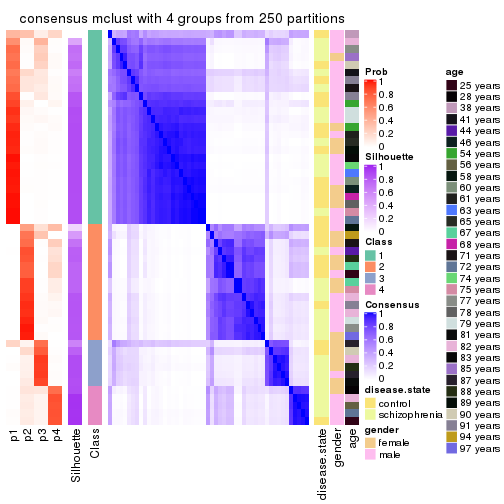
consensus_heatmap(res, k = 5)
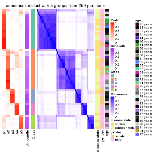
consensus_heatmap(res, k = 6)
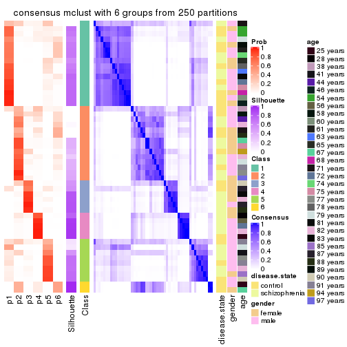
Heatmaps for the membership of samples in all partitions to see how consistent they are:
membership_heatmap(res, k = 2)
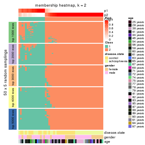
membership_heatmap(res, k = 3)
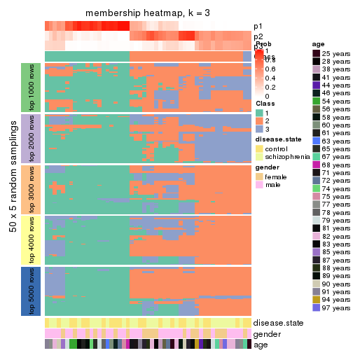
membership_heatmap(res, k = 4)
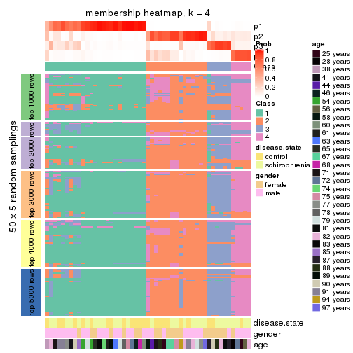
membership_heatmap(res, k = 5)
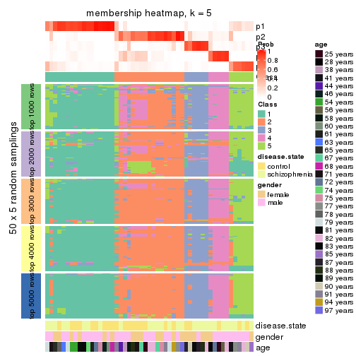
membership_heatmap(res, k = 6)
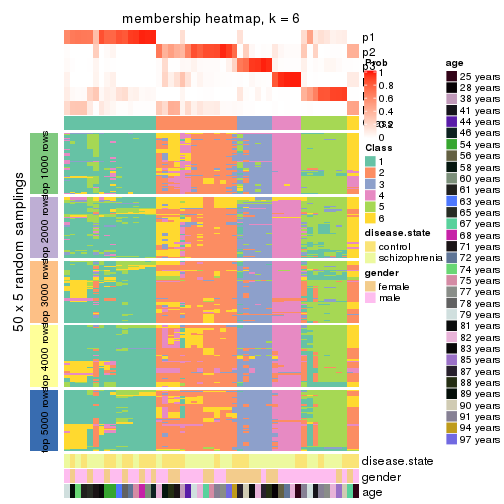
As soon as we have had the classes for columns, we can look for signatures which are significantly different between classes which can be candidate marks for certain classes. Following are the heatmaps for signatures.
Signature heatmaps where rows are scaled:
get_signatures(res, k = 2)
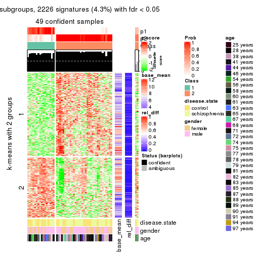
get_signatures(res, k = 3)
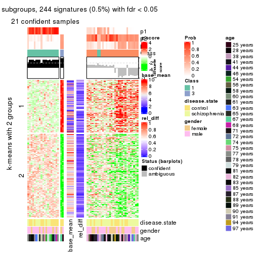
get_signatures(res, k = 4)
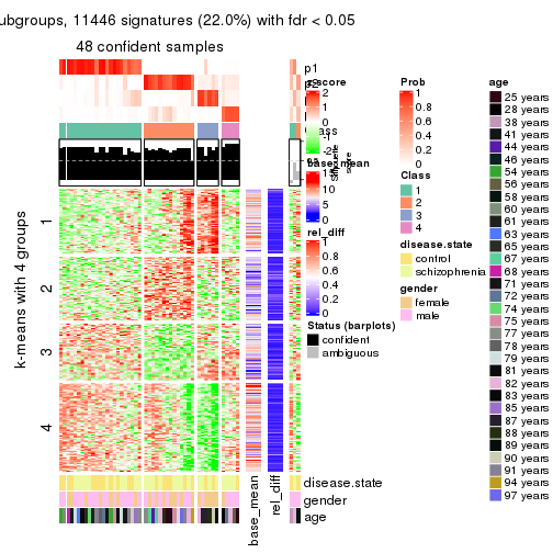
get_signatures(res, k = 5)
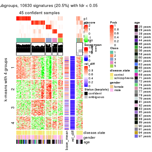
get_signatures(res, k = 6)
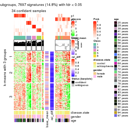
Signature heatmaps where rows are not scaled:
get_signatures(res, k = 2, scale_rows = FALSE)
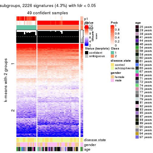
get_signatures(res, k = 3, scale_rows = FALSE)
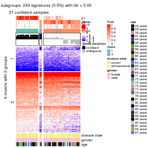
get_signatures(res, k = 4, scale_rows = FALSE)
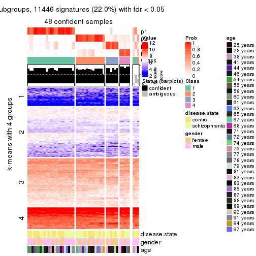
get_signatures(res, k = 5, scale_rows = FALSE)
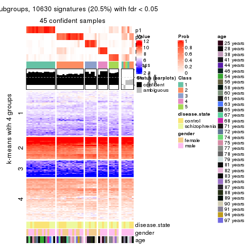
get_signatures(res, k = 6, scale_rows = FALSE)
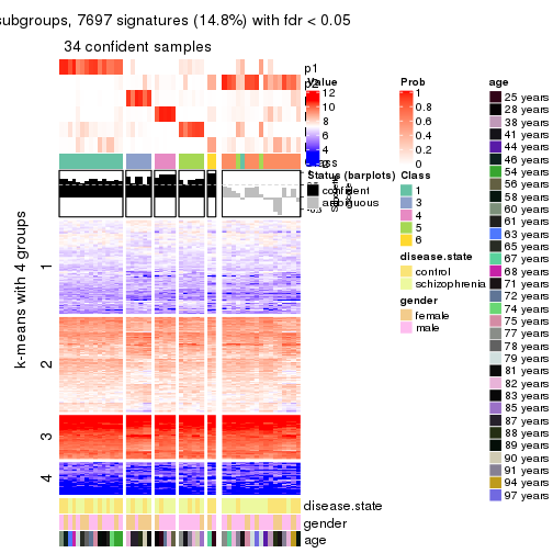
Compare the overlap of signatures from different k:
compare_signatures(res)
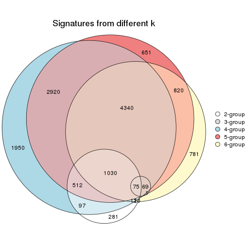
get_signature() returns a data frame invisibly. TO get the list of signatures, the function
call should be assigned to a variable explicitly. In following code, if plot argument is set
to FALSE, no heatmap is plotted while only the differential analysis is performed.
# code only for demonstration
tb = get_signature(res, k = ..., plot = FALSE)
An example of the output of tb is:
#> which_row fdr mean_1 mean_2 scaled_mean_1 scaled_mean_2 km
#> 1 38 0.042760348 8.373488 9.131774 -0.5533452 0.5164555 1
#> 2 40 0.018707592 7.106213 8.469186 -0.6173731 0.5762149 1
#> 3 55 0.019134737 10.221463 11.207825 -0.6159697 0.5749050 1
#> 4 59 0.006059896 5.921854 7.869574 -0.6899429 0.6439467 1
#> 5 60 0.018055526 8.928898 10.211722 -0.6204761 0.5791110 1
#> 6 98 0.009384629 15.714769 14.887706 0.6635654 -0.6193277 2
...
The columns in tb are:
which_row: row indices corresponding to the input matrix.fdr: FDR for the differential test. mean_x: The mean value in group x.scaled_mean_x: The mean value in group x after rows are scaled.km: Row groups if k-means clustering is applied to rows.UMAP plot which shows how samples are separated.
dimension_reduction(res, k = 2, method = "UMAP")
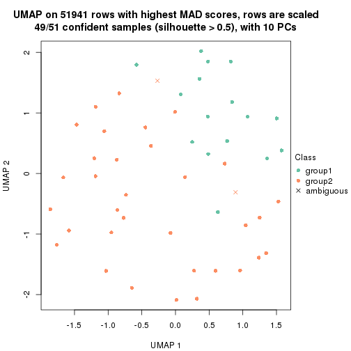
dimension_reduction(res, k = 3, method = "UMAP")
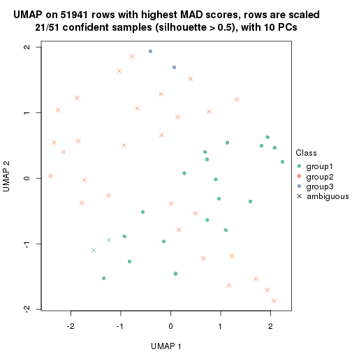
dimension_reduction(res, k = 4, method = "UMAP")
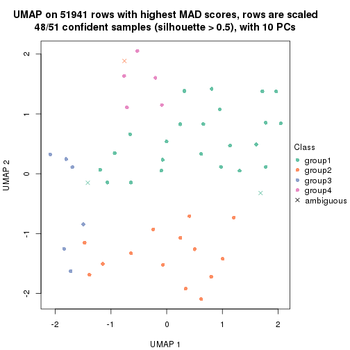
dimension_reduction(res, k = 5, method = "UMAP")
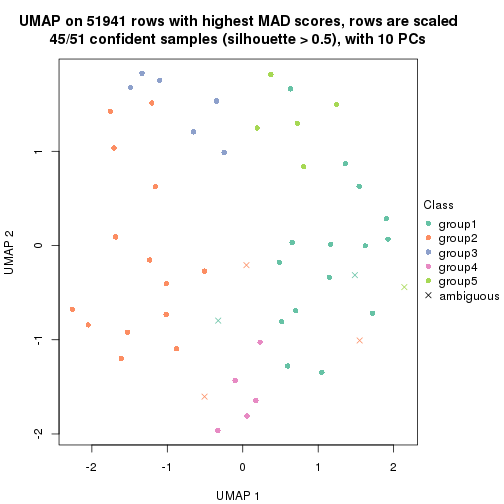
dimension_reduction(res, k = 6, method = "UMAP")
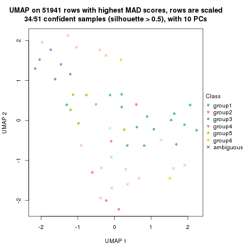
Following heatmap shows how subgroups are split when increasing k:
collect_classes(res)
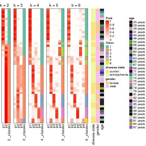
Test correlation between subgroups and known annotations. If the known annotation is numeric, one-way ANOVA test is applied, and if the known annotation is discrete, chi-squared contingency table test is applied.
test_to_known_factors(res)
#> n disease.state(p) gender(p) age(p) k
#> MAD:mclust 49 0.420 0.985 0.202 2
#> MAD:mclust 21 0.688 1.000 0.279 3
#> MAD:mclust 48 0.556 0.077 0.521 4
#> MAD:mclust 45 0.552 0.172 0.598 5
#> MAD:mclust 34 0.228 0.142 0.542 6
If matrix rows can be associated to genes, consider to use functional_enrichment(res,
...) to perform function enrichment for the signature genes. See this vignette for more detailed explanations.
The object with results only for a single top-value method and a single partition method can be extracted as:
res = res_list["MAD", "NMF"]
# you can also extract it by
# res = res_list["MAD:NMF"]
A summary of res and all the functions that can be applied to it:
res
#> A 'ConsensusPartition' object with k = 2, 3, 4, 5, 6.
#> On a matrix with 51941 rows and 51 columns.
#> Top rows (1000, 2000, 3000, 4000, 5000) are extracted by 'MAD' method.
#> Subgroups are detected by 'NMF' method.
#> Performed in total 1250 partitions by row resampling.
#> Best k for subgroups seems to be 2.
#>
#> Following methods can be applied to this 'ConsensusPartition' object:
#> [1] "cola_report" "collect_classes" "collect_plots"
#> [4] "collect_stats" "colnames" "compare_signatures"
#> [7] "consensus_heatmap" "dimension_reduction" "functional_enrichment"
#> [10] "get_anno_col" "get_anno" "get_classes"
#> [13] "get_consensus" "get_matrix" "get_membership"
#> [16] "get_param" "get_signatures" "get_stats"
#> [19] "is_best_k" "is_stable_k" "membership_heatmap"
#> [22] "ncol" "nrow" "plot_ecdf"
#> [25] "rownames" "select_partition_number" "show"
#> [28] "suggest_best_k" "test_to_known_factors"
collect_plots() function collects all the plots made from res for all k (number of partitions)
into one single page to provide an easy and fast comparison between different k.
collect_plots(res)
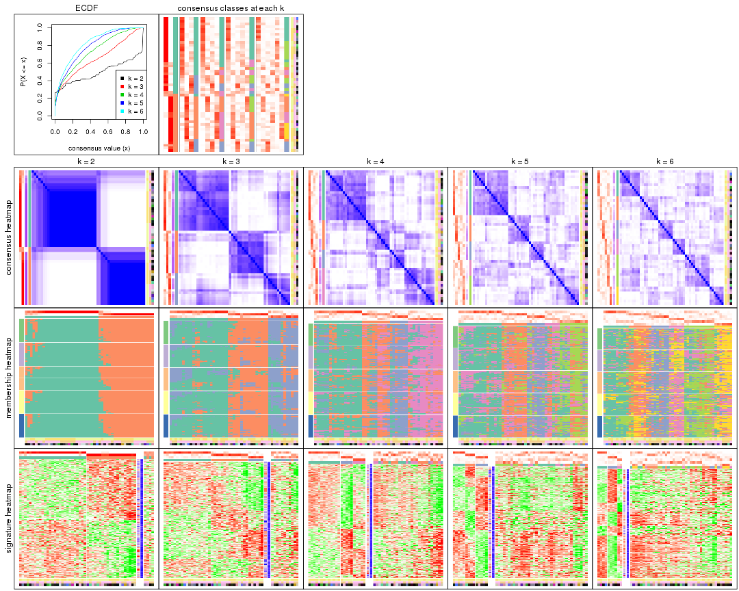
The plots are:
k and the heatmap of
predicted classes for each k.k.k.k.All the plots in panels can be made by individual functions and they are plotted later in this section.
select_partition_number() produces several plots showing different
statistics for choosing “optimized” k. There are following statistics:
k;k, the area increased is defined as \(A_k - A_{k-1}\).The detailed explanations of these statistics can be found in the cola vignette.
Generally speaking, lower PAC score, higher mean silhouette score or higher
concordance corresponds to better partition. Rand index and Jaccard index
measure how similar the current partition is compared to partition with k-1.
If they are too similar, we won't accept k is better than k-1.
select_partition_number(res)
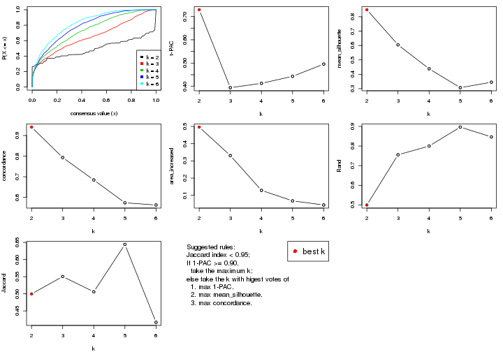
The numeric values for all these statistics can be obtained by get_stats().
get_stats(res)
#> k 1-PAC mean_silhouette concordance area_increased Rand Jaccard
#> 2 2 0.729 0.848 0.941 0.4962 0.500 0.500
#> 3 3 0.395 0.605 0.793 0.3309 0.755 0.550
#> 4 4 0.413 0.438 0.684 0.1289 0.800 0.506
#> 5 5 0.443 0.307 0.574 0.0680 0.896 0.644
#> 6 6 0.496 0.345 0.563 0.0441 0.846 0.417
suggest_best_k() suggests the best \(k\) based on these statistics. The rules are as follows:
suggest_best_k(res)
#> [1] 2
Following shows the table of the partitions (You need to click the show/hide
code output link to see it). The membership matrix (columns with name p*)
is inferred by
clue::cl_consensus()
function with the SE method. Basically the value in the membership matrix
represents the probability to belong to a certain group. The finall class
label for an item is determined with the group with highest probability it
belongs to.
In get_classes() function, the entropy is calculated from the membership
matrix and the silhouette score is calculated from the consensus matrix.
cbind(get_classes(res, k = 2), get_membership(res, k = 2))
#> class entropy silhouette p1 p2
#> GSM439800 1 0.987 0.2420 0.568 0.432
#> GSM439790 1 0.000 0.9336 1.000 0.000
#> GSM439827 2 0.000 0.9308 0.000 1.000
#> GSM439811 2 0.000 0.9308 0.000 1.000
#> GSM439795 2 0.163 0.9155 0.024 0.976
#> GSM439805 1 0.775 0.7026 0.772 0.228
#> GSM439781 1 0.141 0.9213 0.980 0.020
#> GSM439807 2 1.000 -0.0604 0.500 0.500
#> GSM439820 2 0.000 0.9308 0.000 1.000
#> GSM439784 1 0.416 0.8716 0.916 0.084
#> GSM439824 2 0.000 0.9308 0.000 1.000
#> GSM439794 2 0.469 0.8534 0.100 0.900
#> GSM439809 1 0.000 0.9336 1.000 0.000
#> GSM439785 1 0.866 0.5991 0.712 0.288
#> GSM439803 1 0.327 0.8918 0.940 0.060
#> GSM439778 1 0.000 0.9336 1.000 0.000
#> GSM439791 1 0.000 0.9336 1.000 0.000
#> GSM439786 1 0.000 0.9336 1.000 0.000
#> GSM439828 2 0.000 0.9308 0.000 1.000
#> GSM439806 1 0.000 0.9336 1.000 0.000
#> GSM439815 1 0.000 0.9336 1.000 0.000
#> GSM439817 2 0.000 0.9308 0.000 1.000
#> GSM439796 2 0.518 0.8361 0.116 0.884
#> GSM439798 1 0.000 0.9336 1.000 0.000
#> GSM439821 2 0.000 0.9308 0.000 1.000
#> GSM439823 2 0.000 0.9308 0.000 1.000
#> GSM439813 1 0.000 0.9336 1.000 0.000
#> GSM439801 2 0.518 0.8361 0.116 0.884
#> GSM439810 1 0.000 0.9336 1.000 0.000
#> GSM439783 1 0.000 0.9336 1.000 0.000
#> GSM439826 2 0.000 0.9308 0.000 1.000
#> GSM439812 1 0.000 0.9336 1.000 0.000
#> GSM439818 2 0.000 0.9308 0.000 1.000
#> GSM439792 1 0.000 0.9336 1.000 0.000
#> GSM439802 1 0.000 0.9336 1.000 0.000
#> GSM439825 2 0.000 0.9308 0.000 1.000
#> GSM439780 1 0.000 0.9336 1.000 0.000
#> GSM439787 2 0.000 0.9308 0.000 1.000
#> GSM439808 2 0.000 0.9308 0.000 1.000
#> GSM439804 1 0.697 0.7564 0.812 0.188
#> GSM439822 2 0.000 0.9308 0.000 1.000
#> GSM439816 2 0.996 0.0902 0.464 0.536
#> GSM439789 1 0.000 0.9336 1.000 0.000
#> GSM439799 2 0.000 0.9308 0.000 1.000
#> GSM439814 1 0.000 0.9336 1.000 0.000
#> GSM439782 1 0.000 0.9336 1.000 0.000
#> GSM439779 1 0.000 0.9336 1.000 0.000
#> GSM439793 1 0.000 0.9336 1.000 0.000
#> GSM439788 1 0.000 0.9336 1.000 0.000
#> GSM439797 1 0.975 0.3136 0.592 0.408
#> GSM439819 2 0.000 0.9308 0.000 1.000
cbind(get_classes(res, k = 3), get_membership(res, k = 3))
#> class entropy silhouette p1 p2 p3
#> GSM439800 3 0.8693 0.4128 0.232 0.176 0.592
#> GSM439790 1 0.6180 0.3234 0.584 0.000 0.416
#> GSM439827 2 0.2804 0.7987 0.016 0.924 0.060
#> GSM439811 2 0.3637 0.7970 0.024 0.892 0.084
#> GSM439795 3 0.3267 0.5853 0.000 0.116 0.884
#> GSM439805 3 0.1753 0.6602 0.048 0.000 0.952
#> GSM439781 3 0.5529 0.4701 0.296 0.000 0.704
#> GSM439807 3 0.2743 0.6410 0.020 0.052 0.928
#> GSM439820 2 0.4750 0.7184 0.000 0.784 0.216
#> GSM439784 1 0.5260 0.7087 0.828 0.092 0.080
#> GSM439824 2 0.5953 0.5533 0.280 0.708 0.012
#> GSM439794 2 0.7323 0.6167 0.196 0.700 0.104
#> GSM439809 1 0.3551 0.7294 0.868 0.000 0.132
#> GSM439785 1 0.6201 0.6314 0.748 0.208 0.044
#> GSM439803 1 0.6764 0.6723 0.744 0.148 0.108
#> GSM439778 1 0.4605 0.6746 0.796 0.000 0.204
#> GSM439791 1 0.1529 0.7595 0.960 0.000 0.040
#> GSM439786 3 0.5835 0.3760 0.340 0.000 0.660
#> GSM439828 2 0.1765 0.8025 0.004 0.956 0.040
#> GSM439806 1 0.3425 0.7397 0.884 0.004 0.112
#> GSM439815 1 0.4883 0.6860 0.788 0.004 0.208
#> GSM439817 2 0.3155 0.7896 0.044 0.916 0.040
#> GSM439796 2 0.7433 0.5341 0.268 0.660 0.072
#> GSM439798 3 0.4842 0.5681 0.224 0.000 0.776
#> GSM439821 2 0.4702 0.7241 0.000 0.788 0.212
#> GSM439823 2 0.1878 0.8022 0.004 0.952 0.044
#> GSM439813 1 0.3686 0.7256 0.860 0.000 0.140
#> GSM439801 3 0.3340 0.5821 0.000 0.120 0.880
#> GSM439810 1 0.0848 0.7578 0.984 0.008 0.008
#> GSM439783 1 0.3694 0.7540 0.896 0.052 0.052
#> GSM439826 2 0.3528 0.7496 0.092 0.892 0.016
#> GSM439812 1 0.2066 0.7590 0.940 0.000 0.060
#> GSM439818 2 0.3340 0.7834 0.000 0.880 0.120
#> GSM439792 1 0.2229 0.7592 0.944 0.012 0.044
#> GSM439802 3 0.3941 0.6158 0.156 0.000 0.844
#> GSM439825 2 0.3412 0.7790 0.000 0.876 0.124
#> GSM439780 1 0.5905 0.4746 0.648 0.000 0.352
#> GSM439787 3 0.5327 0.3438 0.000 0.272 0.728
#> GSM439808 3 0.6309 -0.2977 0.000 0.500 0.500
#> GSM439804 1 0.6761 0.5793 0.700 0.252 0.048
#> GSM439822 2 0.1337 0.7954 0.012 0.972 0.016
#> GSM439816 1 0.6737 0.3321 0.600 0.384 0.016
#> GSM439789 1 0.3832 0.7177 0.880 0.100 0.020
#> GSM439799 2 0.6516 0.2398 0.004 0.516 0.480
#> GSM439814 1 0.2939 0.7329 0.916 0.072 0.012
#> GSM439782 1 0.5291 0.6079 0.732 0.000 0.268
#> GSM439779 1 0.2096 0.7583 0.944 0.004 0.052
#> GSM439793 3 0.6307 -0.0791 0.488 0.000 0.512
#> GSM439788 1 0.6140 0.3393 0.596 0.000 0.404
#> GSM439797 1 0.8033 0.5310 0.640 0.240 0.120
#> GSM439819 2 0.4750 0.7221 0.000 0.784 0.216
cbind(get_classes(res, k = 4), get_membership(res, k = 4))
#> class entropy silhouette p1 p2 p3 p4
#> GSM439800 4 0.680 0.2062 0.088 0.004 0.384 0.524
#> GSM439790 1 0.539 0.4862 0.632 0.024 0.344 0.000
#> GSM439827 2 0.390 0.4655 0.020 0.840 0.012 0.128
#> GSM439811 2 0.335 0.4803 0.004 0.864 0.016 0.116
#> GSM439795 3 0.436 0.6250 0.000 0.084 0.816 0.100
#> GSM439805 3 0.352 0.6518 0.032 0.076 0.876 0.016
#> GSM439781 2 0.710 0.1313 0.196 0.564 0.240 0.000
#> GSM439807 3 0.418 0.6396 0.020 0.132 0.828 0.020
#> GSM439820 2 0.627 0.4290 0.000 0.664 0.148 0.188
#> GSM439784 2 0.557 0.3255 0.272 0.676 0.052 0.000
#> GSM439824 4 0.848 0.1213 0.220 0.336 0.032 0.412
#> GSM439794 4 0.382 0.5827 0.108 0.000 0.048 0.844
#> GSM439809 1 0.411 0.7008 0.832 0.084 0.084 0.000
#> GSM439785 1 0.835 0.2782 0.500 0.212 0.044 0.244
#> GSM439803 4 0.682 0.3059 0.324 0.000 0.120 0.556
#> GSM439778 1 0.467 0.6471 0.768 0.004 0.200 0.028
#> GSM439791 1 0.245 0.7198 0.912 0.072 0.016 0.000
#> GSM439786 3 0.750 0.0393 0.368 0.184 0.448 0.000
#> GSM439828 2 0.567 0.1398 0.012 0.588 0.012 0.388
#> GSM439806 1 0.561 0.4742 0.628 0.336 0.036 0.000
#> GSM439815 1 0.685 0.4999 0.596 0.008 0.284 0.112
#> GSM439817 2 0.630 0.0209 0.012 0.532 0.036 0.420
#> GSM439796 4 0.409 0.5832 0.116 0.008 0.040 0.836
#> GSM439798 2 0.742 -0.1672 0.168 0.436 0.396 0.000
#> GSM439821 4 0.667 0.2624 0.000 0.252 0.140 0.608
#> GSM439823 4 0.367 0.5249 0.000 0.164 0.012 0.824
#> GSM439813 1 0.377 0.6896 0.840 0.008 0.136 0.016
#> GSM439801 3 0.531 0.5944 0.000 0.144 0.748 0.108
#> GSM439810 1 0.259 0.7143 0.920 0.040 0.028 0.012
#> GSM439783 1 0.459 0.6703 0.804 0.004 0.064 0.128
#> GSM439826 4 0.534 0.4996 0.032 0.180 0.032 0.756
#> GSM439812 1 0.290 0.7214 0.904 0.056 0.032 0.008
#> GSM439818 4 0.355 0.5483 0.000 0.096 0.044 0.860
#> GSM439792 1 0.386 0.6800 0.824 0.152 0.024 0.000
#> GSM439802 3 0.409 0.5357 0.172 0.000 0.804 0.024
#> GSM439825 4 0.511 0.4456 0.000 0.196 0.060 0.744
#> GSM439780 1 0.557 0.4142 0.584 0.008 0.396 0.012
#> GSM439787 3 0.539 0.2447 0.000 0.400 0.584 0.016
#> GSM439808 2 0.691 0.0599 0.000 0.520 0.364 0.116
#> GSM439804 4 0.559 0.4965 0.260 0.004 0.048 0.688
#> GSM439822 4 0.358 0.5138 0.000 0.180 0.004 0.816
#> GSM439816 4 0.797 0.1948 0.392 0.124 0.036 0.448
#> GSM439789 1 0.495 0.6318 0.800 0.036 0.040 0.124
#> GSM439799 4 0.519 0.4109 0.004 0.020 0.292 0.684
#> GSM439814 1 0.444 0.6817 0.836 0.084 0.036 0.044
#> GSM439782 1 0.570 0.5813 0.688 0.008 0.256 0.048
#> GSM439779 1 0.380 0.7117 0.848 0.112 0.036 0.004
#> GSM439793 2 0.750 0.0644 0.324 0.476 0.200 0.000
#> GSM439788 1 0.672 0.5184 0.616 0.204 0.180 0.000
#> GSM439797 1 0.729 0.2179 0.488 0.412 0.036 0.064
#> GSM439819 2 0.702 0.3210 0.000 0.544 0.144 0.312
cbind(get_classes(res, k = 5), get_membership(res, k = 5))
#> class entropy silhouette p1 p2 p3 p4 p5
#> GSM439800 3 0.746 0.08861 0.028 0.292 0.408 0.268 0.004
#> GSM439790 1 0.750 0.19346 0.400 0.000 0.228 0.328 0.044
#> GSM439827 5 0.479 0.37026 0.032 0.204 0.004 0.024 0.736
#> GSM439811 5 0.421 0.38923 0.020 0.184 0.012 0.008 0.776
#> GSM439795 3 0.263 0.63437 0.000 0.080 0.892 0.016 0.012
#> GSM439805 3 0.425 0.60998 0.012 0.036 0.824 0.068 0.060
#> GSM439781 5 0.845 -0.00557 0.228 0.000 0.204 0.216 0.352
#> GSM439807 3 0.586 0.51830 0.048 0.012 0.708 0.116 0.116
#> GSM439820 5 0.685 0.31672 0.040 0.092 0.132 0.084 0.652
#> GSM439784 5 0.582 0.25124 0.296 0.012 0.028 0.040 0.624
#> GSM439824 2 0.773 0.14666 0.240 0.468 0.004 0.076 0.212
#> GSM439794 2 0.640 0.35675 0.060 0.624 0.084 0.228 0.004
#> GSM439809 1 0.445 0.52957 0.800 0.000 0.084 0.064 0.052
#> GSM439785 4 0.790 0.20758 0.272 0.144 0.004 0.456 0.124
#> GSM439803 4 0.753 0.08083 0.192 0.344 0.056 0.408 0.000
#> GSM439778 1 0.650 0.39304 0.572 0.016 0.132 0.272 0.008
#> GSM439791 1 0.275 0.54861 0.900 0.008 0.012 0.048 0.032
#> GSM439786 4 0.818 0.03606 0.208 0.000 0.188 0.420 0.184
#> GSM439828 5 0.532 0.03667 0.004 0.408 0.000 0.044 0.544
#> GSM439806 1 0.669 0.27657 0.552 0.004 0.024 0.148 0.272
#> GSM439815 4 0.757 -0.01287 0.328 0.032 0.228 0.404 0.008
#> GSM439817 5 0.702 0.04321 0.028 0.332 0.008 0.140 0.492
#> GSM439796 2 0.617 0.28535 0.040 0.552 0.060 0.348 0.000
#> GSM439798 5 0.802 0.07036 0.112 0.000 0.208 0.268 0.412
#> GSM439821 2 0.665 0.35083 0.000 0.580 0.156 0.040 0.224
#> GSM439823 2 0.668 0.44660 0.004 0.556 0.028 0.276 0.136
#> GSM439813 1 0.595 0.39466 0.644 0.004 0.144 0.196 0.012
#> GSM439801 3 0.588 0.56164 0.000 0.072 0.688 0.088 0.152
#> GSM439810 1 0.261 0.53499 0.904 0.032 0.000 0.040 0.024
#> GSM439783 1 0.743 0.29486 0.536 0.140 0.064 0.244 0.016
#> GSM439826 2 0.438 0.51777 0.036 0.796 0.000 0.052 0.116
#> GSM439812 1 0.538 0.43432 0.728 0.008 0.048 0.164 0.052
#> GSM439818 2 0.322 0.57556 0.000 0.872 0.048 0.028 0.052
#> GSM439792 1 0.485 0.51530 0.772 0.008 0.028 0.124 0.068
#> GSM439802 3 0.383 0.55238 0.044 0.000 0.812 0.136 0.008
#> GSM439825 2 0.486 0.51533 0.000 0.760 0.092 0.028 0.120
#> GSM439780 1 0.663 0.33232 0.500 0.000 0.292 0.200 0.008
#> GSM439787 3 0.576 0.27003 0.000 0.044 0.540 0.024 0.392
#> GSM439808 5 0.733 -0.12119 0.012 0.072 0.396 0.084 0.436
#> GSM439804 4 0.678 -0.15360 0.120 0.408 0.032 0.440 0.000
#> GSM439822 2 0.277 0.54503 0.000 0.864 0.008 0.004 0.124
#> GSM439816 1 0.672 -0.03327 0.468 0.392 0.000 0.100 0.040
#> GSM439789 1 0.446 0.45218 0.768 0.072 0.000 0.152 0.008
#> GSM439799 2 0.691 0.23497 0.000 0.420 0.244 0.328 0.008
#> GSM439814 1 0.443 0.46241 0.792 0.032 0.004 0.132 0.040
#> GSM439782 1 0.672 0.29982 0.476 0.004 0.168 0.344 0.008
#> GSM439779 1 0.279 0.54917 0.892 0.000 0.020 0.060 0.028
#> GSM439793 5 0.794 0.14998 0.204 0.000 0.224 0.124 0.448
#> GSM439788 1 0.766 0.29968 0.508 0.000 0.168 0.164 0.160
#> GSM439797 4 0.795 0.10733 0.256 0.036 0.020 0.368 0.320
#> GSM439819 5 0.652 0.19802 0.000 0.284 0.116 0.036 0.564
cbind(get_classes(res, k = 6), get_membership(res, k = 6))
#> class entropy silhouette p1 p2 p3 p4 p5 p6
#> GSM439800 3 0.767 0.2160 0.068 0.016 0.452 0.296 0.056 0.112
#> GSM439790 5 0.454 0.4452 0.076 0.020 0.100 0.032 0.772 0.000
#> GSM439827 2 0.479 0.3633 0.020 0.624 0.000 0.012 0.016 0.328
#> GSM439811 2 0.485 0.3767 0.008 0.624 0.008 0.012 0.020 0.328
#> GSM439795 3 0.284 0.6391 0.016 0.008 0.888 0.052 0.020 0.016
#> GSM439805 3 0.436 0.6141 0.004 0.048 0.784 0.020 0.120 0.024
#> GSM439781 5 0.641 0.3065 0.036 0.260 0.128 0.016 0.556 0.004
#> GSM439807 3 0.698 0.4526 0.168 0.116 0.576 0.084 0.052 0.004
#> GSM439820 2 0.789 0.3168 0.196 0.484 0.104 0.120 0.008 0.088
#> GSM439784 2 0.694 0.2406 0.160 0.552 0.048 0.004 0.192 0.044
#> GSM439824 6 0.619 0.3292 0.180 0.124 0.000 0.048 0.028 0.620
#> GSM439794 4 0.754 0.4126 0.072 0.008 0.072 0.456 0.088 0.304
#> GSM439809 1 0.436 0.5479 0.764 0.052 0.028 0.008 0.148 0.000
#> GSM439785 5 0.694 0.1866 0.048 0.116 0.000 0.324 0.472 0.040
#> GSM439803 4 0.696 0.4641 0.096 0.004 0.008 0.520 0.216 0.156
#> GSM439778 5 0.612 0.2920 0.244 0.008 0.116 0.040 0.588 0.004
#> GSM439791 1 0.502 0.4302 0.632 0.056 0.000 0.016 0.292 0.004
#> GSM439786 5 0.626 0.4111 0.036 0.108 0.052 0.184 0.620 0.000
#> GSM439828 2 0.582 0.2643 0.016 0.556 0.000 0.092 0.016 0.320
#> GSM439806 1 0.712 0.0897 0.368 0.252 0.008 0.024 0.332 0.016
#> GSM439815 1 0.704 0.2307 0.524 0.028 0.136 0.252 0.044 0.016
#> GSM439817 2 0.789 0.1635 0.092 0.384 0.016 0.208 0.020 0.280
#> GSM439796 4 0.500 0.5369 0.036 0.000 0.028 0.628 0.004 0.304
#> GSM439798 5 0.671 0.1943 0.016 0.324 0.092 0.080 0.488 0.000
#> GSM439821 6 0.737 0.2158 0.000 0.192 0.244 0.112 0.012 0.440
#> GSM439823 4 0.660 0.3262 0.028 0.136 0.008 0.528 0.020 0.280
#> GSM439813 1 0.388 0.5309 0.824 0.020 0.064 0.056 0.036 0.000
#> GSM439801 3 0.598 0.5441 0.000 0.100 0.656 0.132 0.092 0.020
#> GSM439810 1 0.592 0.4715 0.624 0.040 0.004 0.024 0.240 0.068
#> GSM439783 5 0.816 0.1190 0.272 0.020 0.060 0.072 0.400 0.176
#> GSM439826 6 0.416 0.4230 0.044 0.052 0.000 0.112 0.004 0.788
#> GSM439812 1 0.342 0.5497 0.860 0.032 0.028 0.052 0.016 0.012
#> GSM439818 6 0.510 0.3871 0.004 0.028 0.116 0.128 0.008 0.716
#> GSM439792 5 0.658 -0.0585 0.404 0.052 0.012 0.040 0.456 0.036
#> GSM439802 3 0.601 0.5794 0.088 0.024 0.684 0.072 0.112 0.020
#> GSM439825 6 0.464 0.4419 0.000 0.036 0.164 0.052 0.008 0.740
#> GSM439780 5 0.733 0.0264 0.340 0.012 0.220 0.052 0.368 0.008
#> GSM439787 3 0.543 0.3675 0.008 0.292 0.620 0.016 0.016 0.048
#> GSM439808 2 0.766 -0.0831 0.096 0.404 0.352 0.092 0.016 0.040
#> GSM439804 4 0.562 0.5859 0.096 0.000 0.000 0.648 0.072 0.184
#> GSM439822 6 0.370 0.4568 0.000 0.048 0.024 0.108 0.004 0.816
#> GSM439816 6 0.664 0.1339 0.352 0.020 0.000 0.104 0.052 0.472
#> GSM439789 1 0.629 0.2671 0.528 0.016 0.000 0.100 0.316 0.040
#> GSM439799 4 0.540 0.4818 0.000 0.044 0.100 0.704 0.024 0.128
#> GSM439814 1 0.318 0.5676 0.872 0.024 0.004 0.040 0.024 0.036
#> GSM439782 5 0.590 0.3426 0.228 0.012 0.060 0.080 0.620 0.000
#> GSM439779 1 0.512 0.3756 0.616 0.028 0.012 0.020 0.320 0.004
#> GSM439793 2 0.710 -0.0304 0.100 0.440 0.080 0.024 0.352 0.004
#> GSM439788 5 0.582 0.3775 0.200 0.080 0.060 0.016 0.644 0.000
#> GSM439797 5 0.624 0.3330 0.020 0.244 0.008 0.176 0.548 0.004
#> GSM439819 2 0.588 0.3306 0.000 0.600 0.112 0.036 0.008 0.244
Heatmaps for the consensus matrix. It visualizes the probability of two samples to be in a same group.
consensus_heatmap(res, k = 2)
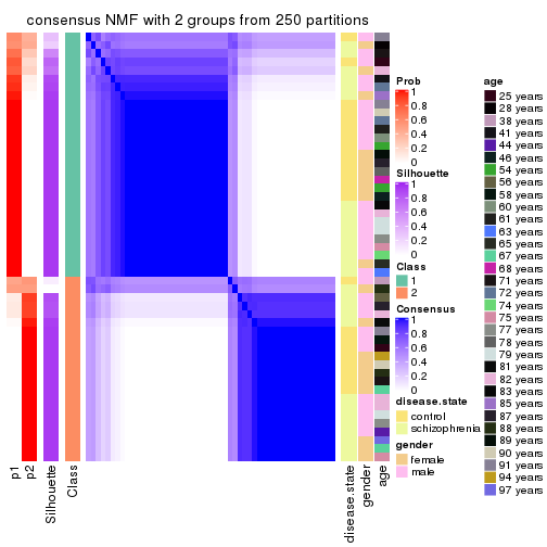
consensus_heatmap(res, k = 3)
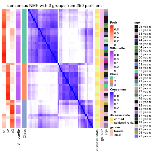
consensus_heatmap(res, k = 4)
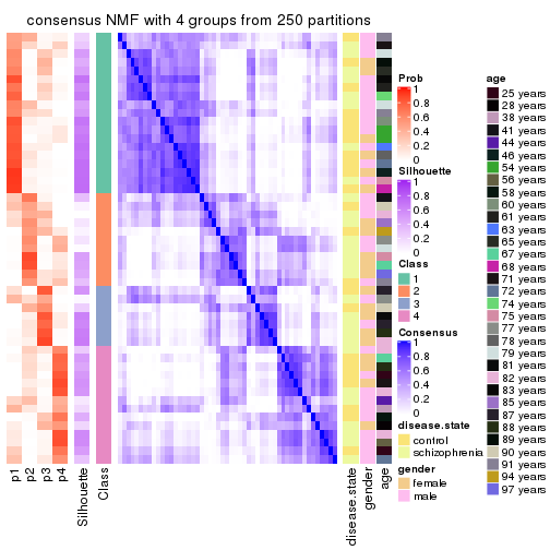
consensus_heatmap(res, k = 5)
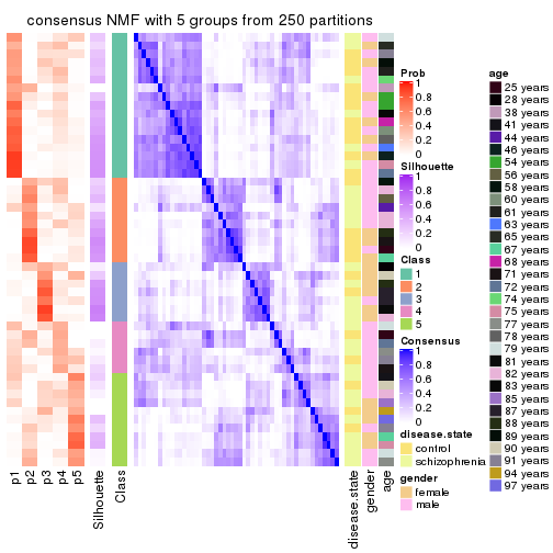
consensus_heatmap(res, k = 6)
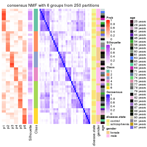
Heatmaps for the membership of samples in all partitions to see how consistent they are:
membership_heatmap(res, k = 2)
membership_heatmap(res, k = 3)
membership_heatmap(res, k = 4)
membership_heatmap(res, k = 5)
membership_heatmap(res, k = 6)
As soon as we have had the classes for columns, we can look for signatures which are significantly different between classes which can be candidate marks for certain classes. Following are the heatmaps for signatures.
Signature heatmaps where rows are scaled:
get_signatures(res, k = 2)
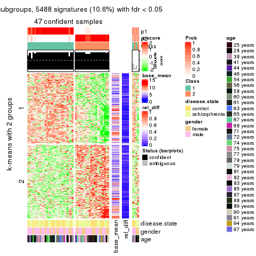
get_signatures(res, k = 3)
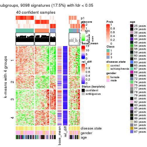
get_signatures(res, k = 4)
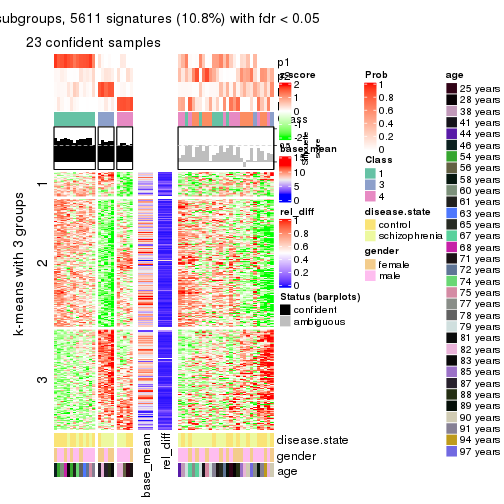
get_signatures(res, k = 5)
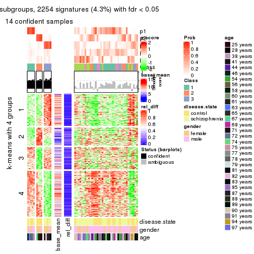
get_signatures(res, k = 6)
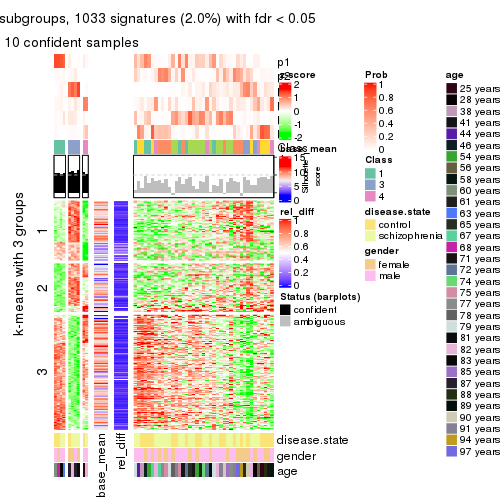
Signature heatmaps where rows are not scaled:
get_signatures(res, k = 2, scale_rows = FALSE)

get_signatures(res, k = 3, scale_rows = FALSE)
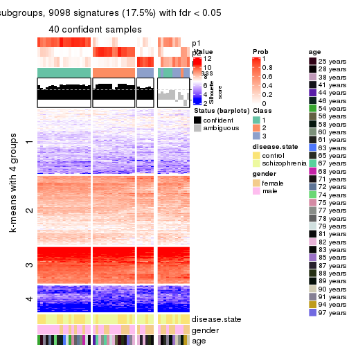
get_signatures(res, k = 4, scale_rows = FALSE)
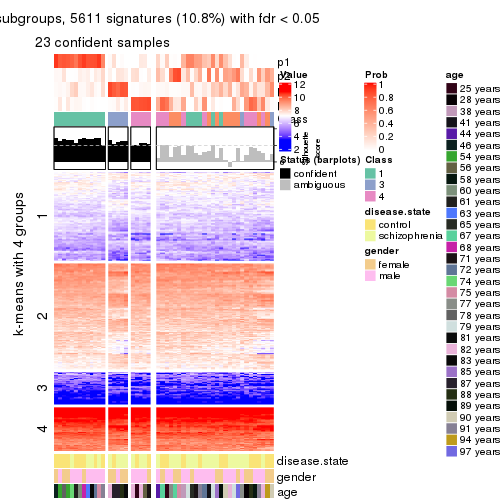
get_signatures(res, k = 5, scale_rows = FALSE)
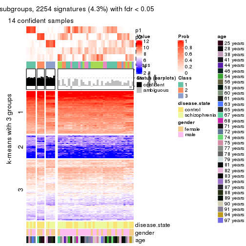
get_signatures(res, k = 6, scale_rows = FALSE)
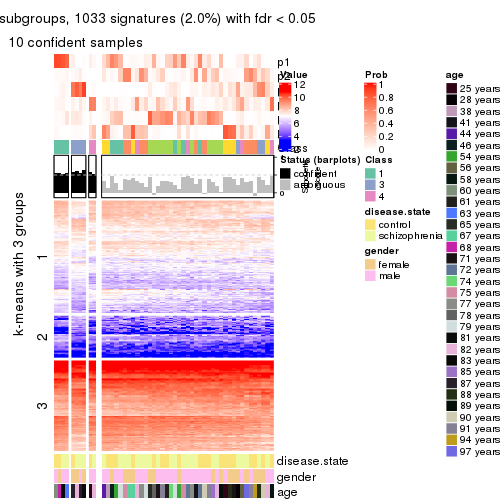
Compare the overlap of signatures from different k:
compare_signatures(res)
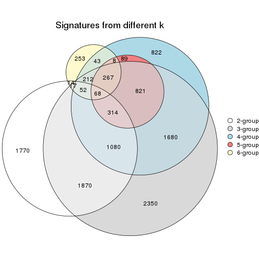
get_signature() returns a data frame invisibly. TO get the list of signatures, the function
call should be assigned to a variable explicitly. In following code, if plot argument is set
to FALSE, no heatmap is plotted while only the differential analysis is performed.
# code only for demonstration
tb = get_signature(res, k = ..., plot = FALSE)
An example of the output of tb is:
#> which_row fdr mean_1 mean_2 scaled_mean_1 scaled_mean_2 km
#> 1 38 0.042760348 8.373488 9.131774 -0.5533452 0.5164555 1
#> 2 40 0.018707592 7.106213 8.469186 -0.6173731 0.5762149 1
#> 3 55 0.019134737 10.221463 11.207825 -0.6159697 0.5749050 1
#> 4 59 0.006059896 5.921854 7.869574 -0.6899429 0.6439467 1
#> 5 60 0.018055526 8.928898 10.211722 -0.6204761 0.5791110 1
#> 6 98 0.009384629 15.714769 14.887706 0.6635654 -0.6193277 2
...
The columns in tb are:
which_row: row indices corresponding to the input matrix.fdr: FDR for the differential test. mean_x: The mean value in group x.scaled_mean_x: The mean value in group x after rows are scaled.km: Row groups if k-means clustering is applied to rows.UMAP plot which shows how samples are separated.
dimension_reduction(res, k = 2, method = "UMAP")
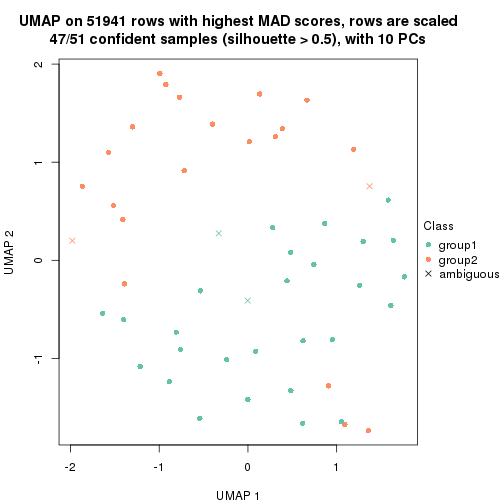
dimension_reduction(res, k = 3, method = "UMAP")
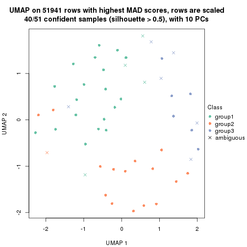
dimension_reduction(res, k = 4, method = "UMAP")
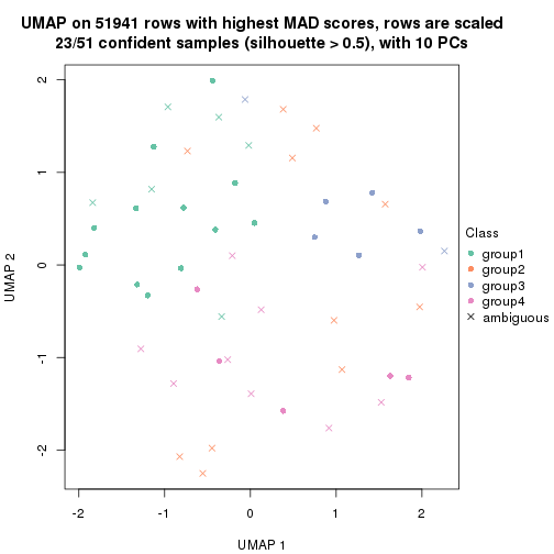
dimension_reduction(res, k = 5, method = "UMAP")
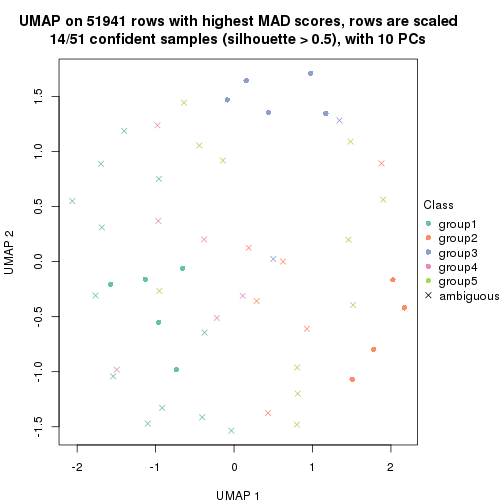
dimension_reduction(res, k = 6, method = "UMAP")
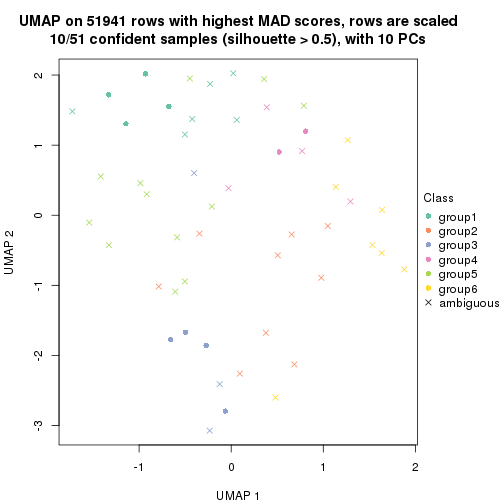
Following heatmap shows how subgroups are split when increasing k:
collect_classes(res)
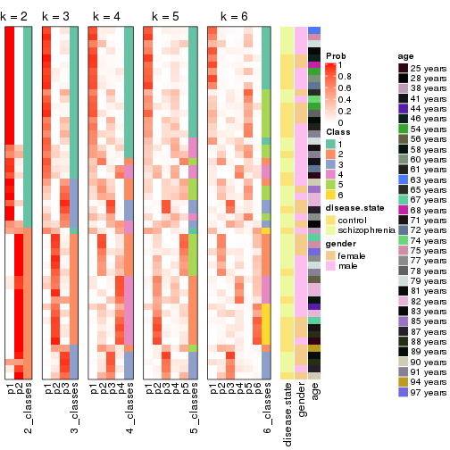
Test correlation between subgroups and known annotations. If the known annotation is numeric, one-way ANOVA test is applied, and if the known annotation is discrete, chi-squared contingency table test is applied.
test_to_known_factors(res)
#> n disease.state(p) gender(p) age(p) k
#> MAD:NMF 47 0.7958 0.6100 0.723 2
#> MAD:NMF 40 0.2343 0.1089 0.342 3
#> MAD:NMF 23 0.1432 0.0975 0.302 4
#> MAD:NMF 14 0.0541 0.3638 0.304 5
#> MAD:NMF 10 0.7316 0.1534 0.298 6
If matrix rows can be associated to genes, consider to use functional_enrichment(res,
...) to perform function enrichment for the signature genes. See this vignette for more detailed explanations.
The object with results only for a single top-value method and a single partition method can be extracted as:
res = res_list["ATC", "hclust"]
# you can also extract it by
# res = res_list["ATC:hclust"]
A summary of res and all the functions that can be applied to it:
res
#> A 'ConsensusPartition' object with k = 2, 3, 4, 5, 6.
#> On a matrix with 51941 rows and 51 columns.
#> Top rows (1000, 2000, 3000, 4000, 5000) are extracted by 'ATC' method.
#> Subgroups are detected by 'hclust' method.
#> Performed in total 1250 partitions by row resampling.
#> Best k for subgroups seems to be 4.
#>
#> Following methods can be applied to this 'ConsensusPartition' object:
#> [1] "cola_report" "collect_classes" "collect_plots"
#> [4] "collect_stats" "colnames" "compare_signatures"
#> [7] "consensus_heatmap" "dimension_reduction" "functional_enrichment"
#> [10] "get_anno_col" "get_anno" "get_classes"
#> [13] "get_consensus" "get_matrix" "get_membership"
#> [16] "get_param" "get_signatures" "get_stats"
#> [19] "is_best_k" "is_stable_k" "membership_heatmap"
#> [22] "ncol" "nrow" "plot_ecdf"
#> [25] "rownames" "select_partition_number" "show"
#> [28] "suggest_best_k" "test_to_known_factors"
collect_plots() function collects all the plots made from res for all k (number of partitions)
into one single page to provide an easy and fast comparison between different k.
collect_plots(res)
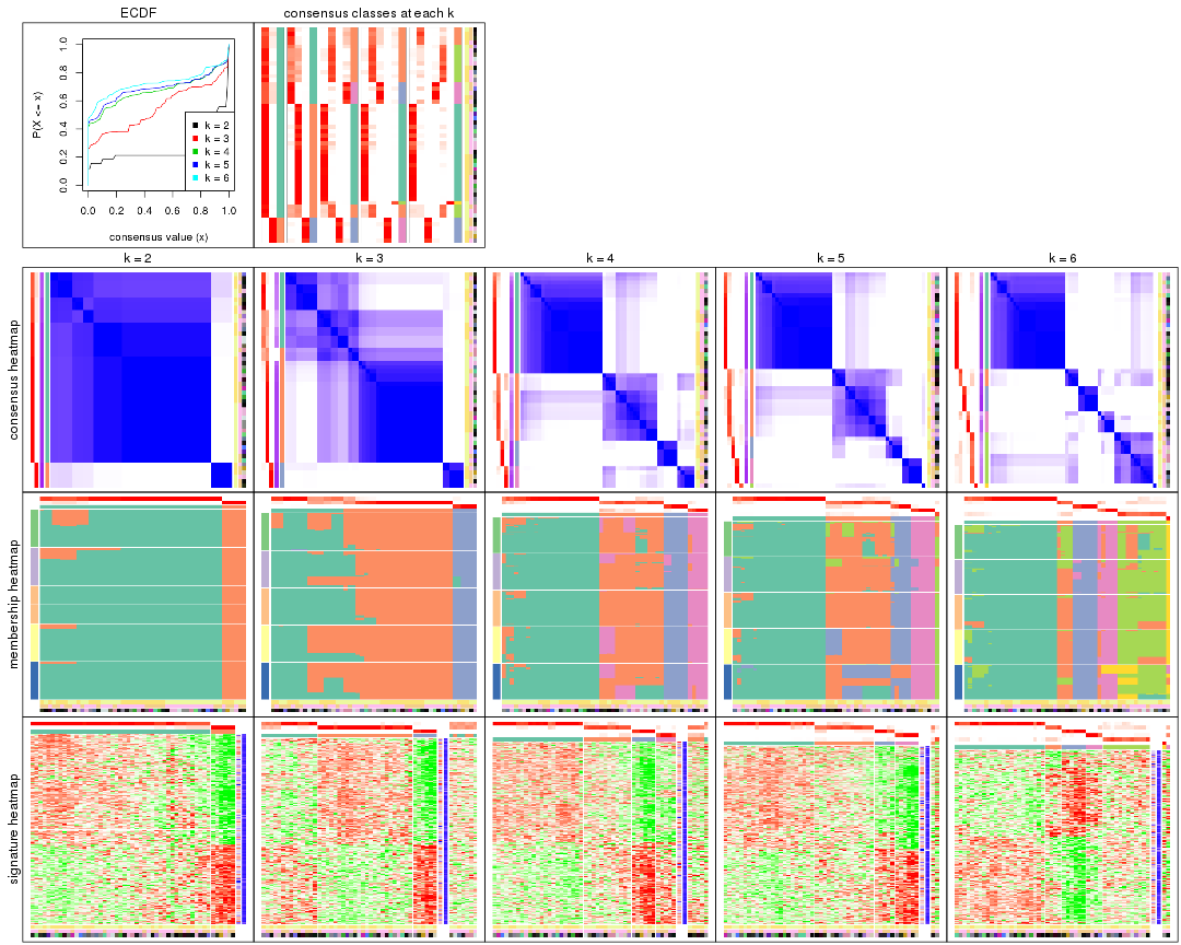
The plots are:
k and the heatmap of
predicted classes for each k.k.k.k.All the plots in panels can be made by individual functions and they are plotted later in this section.
select_partition_number() produces several plots showing different
statistics for choosing “optimized” k. There are following statistics:
k;k, the area increased is defined as \(A_k - A_{k-1}\).The detailed explanations of these statistics can be found in the cola vignette.
Generally speaking, lower PAC score, higher mean silhouette score or higher
concordance corresponds to better partition. Rand index and Jaccard index
measure how similar the current partition is compared to partition with k-1.
If they are too similar, we won't accept k is better than k-1.
select_partition_number(res)
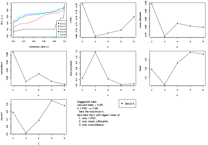
The numeric values for all these statistics can be obtained by get_stats().
get_stats(res)
#> k 1-PAC mean_silhouette concordance area_increased Rand Jaccard
#> 2 2 0.785 0.943 0.965 0.2520 0.788 0.788
#> 3 3 0.681 0.742 0.891 1.1731 0.619 0.516
#> 4 4 0.691 0.822 0.910 0.2279 0.862 0.685
#> 5 5 0.700 0.805 0.891 0.0268 0.982 0.945
#> 6 6 0.743 0.797 0.884 0.0519 0.962 0.879
suggest_best_k() suggests the best \(k\) based on these statistics. The rules are as follows:
suggest_best_k(res)
#> [1] 4
Following shows the table of the partitions (You need to click the show/hide
code output link to see it). The membership matrix (columns with name p*)
is inferred by
clue::cl_consensus()
function with the SE method. Basically the value in the membership matrix
represents the probability to belong to a certain group. The finall class
label for an item is determined with the group with highest probability it
belongs to.
In get_classes() function, the entropy is calculated from the membership
matrix and the silhouette score is calculated from the consensus matrix.
cbind(get_classes(res, k = 2), get_membership(res, k = 2))
#> class entropy silhouette p1 p2
#> GSM439800 1 0.4562 0.905 0.904 0.096
#> GSM439790 1 0.0000 0.960 1.000 0.000
#> GSM439827 1 0.0000 0.960 1.000 0.000
#> GSM439811 1 0.0938 0.957 0.988 0.012
#> GSM439795 2 0.0000 1.000 0.000 1.000
#> GSM439805 1 0.6973 0.827 0.812 0.188
#> GSM439781 1 0.4431 0.908 0.908 0.092
#> GSM439807 2 0.0000 1.000 0.000 1.000
#> GSM439820 1 0.6801 0.835 0.820 0.180
#> GSM439784 1 0.0938 0.957 0.988 0.012
#> GSM439824 1 0.0000 0.960 1.000 0.000
#> GSM439794 1 0.0938 0.957 0.988 0.012
#> GSM439809 1 0.0000 0.960 1.000 0.000
#> GSM439785 1 0.0000 0.960 1.000 0.000
#> GSM439803 1 0.0000 0.960 1.000 0.000
#> GSM439778 1 0.0000 0.960 1.000 0.000
#> GSM439791 1 0.0000 0.960 1.000 0.000
#> GSM439786 1 0.0000 0.960 1.000 0.000
#> GSM439828 1 0.0000 0.960 1.000 0.000
#> GSM439806 1 0.0000 0.960 1.000 0.000
#> GSM439815 1 0.0938 0.957 0.988 0.012
#> GSM439817 1 0.0938 0.957 0.988 0.012
#> GSM439796 1 0.0000 0.960 1.000 0.000
#> GSM439798 1 0.4431 0.908 0.908 0.092
#> GSM439821 2 0.0000 1.000 0.000 1.000
#> GSM439823 1 0.0000 0.960 1.000 0.000
#> GSM439813 1 0.0000 0.960 1.000 0.000
#> GSM439801 1 0.6973 0.827 0.812 0.188
#> GSM439810 1 0.0000 0.960 1.000 0.000
#> GSM439783 1 0.0000 0.960 1.000 0.000
#> GSM439826 1 0.0000 0.960 1.000 0.000
#> GSM439812 1 0.0000 0.960 1.000 0.000
#> GSM439818 1 0.6801 0.835 0.820 0.180
#> GSM439792 1 0.0000 0.960 1.000 0.000
#> GSM439802 1 0.6973 0.827 0.812 0.188
#> GSM439825 1 0.4690 0.903 0.900 0.100
#> GSM439780 1 0.0938 0.957 0.988 0.012
#> GSM439787 2 0.0000 1.000 0.000 1.000
#> GSM439808 2 0.0000 1.000 0.000 1.000
#> GSM439804 1 0.0000 0.960 1.000 0.000
#> GSM439822 1 0.4562 0.905 0.904 0.096
#> GSM439816 1 0.0000 0.960 1.000 0.000
#> GSM439789 1 0.0000 0.960 1.000 0.000
#> GSM439799 1 0.6973 0.827 0.812 0.188
#> GSM439814 1 0.0000 0.960 1.000 0.000
#> GSM439782 1 0.0000 0.960 1.000 0.000
#> GSM439779 1 0.0938 0.957 0.988 0.012
#> GSM439793 1 0.4431 0.908 0.908 0.092
#> GSM439788 1 0.0938 0.957 0.988 0.012
#> GSM439797 1 0.0000 0.960 1.000 0.000
#> GSM439819 2 0.0000 1.000 0.000 1.000
cbind(get_classes(res, k = 3), get_membership(res, k = 3))
#> class entropy silhouette p1 p2 p3
#> GSM439800 1 0.2796 0.6973 0.908 0.092 0.000
#> GSM439790 2 0.0000 0.9116 0.000 1.000 0.000
#> GSM439827 2 0.1964 0.8652 0.056 0.944 0.000
#> GSM439811 2 0.6260 -0.1926 0.448 0.552 0.000
#> GSM439795 3 0.0000 0.9791 0.000 0.000 1.000
#> GSM439805 1 0.0424 0.6567 0.992 0.000 0.008
#> GSM439781 1 0.5465 0.6676 0.712 0.288 0.000
#> GSM439807 3 0.2066 0.9568 0.060 0.000 0.940
#> GSM439820 1 0.0000 0.6602 1.000 0.000 0.000
#> GSM439784 1 0.6291 0.4202 0.532 0.468 0.000
#> GSM439824 2 0.0000 0.9116 0.000 1.000 0.000
#> GSM439794 1 0.6299 0.3993 0.524 0.476 0.000
#> GSM439809 2 0.0000 0.9116 0.000 1.000 0.000
#> GSM439785 2 0.0000 0.9116 0.000 1.000 0.000
#> GSM439803 2 0.2448 0.8410 0.076 0.924 0.000
#> GSM439778 2 0.0000 0.9116 0.000 1.000 0.000
#> GSM439791 2 0.6154 -0.0273 0.408 0.592 0.000
#> GSM439786 2 0.0237 0.9090 0.004 0.996 0.000
#> GSM439828 2 0.1529 0.8811 0.040 0.960 0.000
#> GSM439806 2 0.0000 0.9116 0.000 1.000 0.000
#> GSM439815 2 0.6260 -0.1926 0.448 0.552 0.000
#> GSM439817 1 0.6280 0.4386 0.540 0.460 0.000
#> GSM439796 2 0.3340 0.7786 0.120 0.880 0.000
#> GSM439798 1 0.5465 0.6676 0.712 0.288 0.000
#> GSM439821 3 0.0000 0.9791 0.000 0.000 1.000
#> GSM439823 2 0.1529 0.8811 0.040 0.960 0.000
#> GSM439813 2 0.0000 0.9116 0.000 1.000 0.000
#> GSM439801 1 0.0424 0.6567 0.992 0.000 0.008
#> GSM439810 2 0.0000 0.9116 0.000 1.000 0.000
#> GSM439783 2 0.0000 0.9116 0.000 1.000 0.000
#> GSM439826 2 0.0000 0.9116 0.000 1.000 0.000
#> GSM439812 2 0.0000 0.9116 0.000 1.000 0.000
#> GSM439818 1 0.0000 0.6602 1.000 0.000 0.000
#> GSM439792 2 0.0000 0.9116 0.000 1.000 0.000
#> GSM439802 1 0.0424 0.6567 0.992 0.000 0.008
#> GSM439825 1 0.2537 0.6935 0.920 0.080 0.000
#> GSM439780 1 0.6008 0.5937 0.628 0.372 0.000
#> GSM439787 3 0.0000 0.9791 0.000 0.000 1.000
#> GSM439808 3 0.0000 0.9791 0.000 0.000 1.000
#> GSM439804 2 0.0000 0.9116 0.000 1.000 0.000
#> GSM439822 1 0.2711 0.6961 0.912 0.088 0.000
#> GSM439816 2 0.0000 0.9116 0.000 1.000 0.000
#> GSM439789 2 0.0000 0.9116 0.000 1.000 0.000
#> GSM439799 1 0.0424 0.6567 0.992 0.000 0.008
#> GSM439814 2 0.0000 0.9116 0.000 1.000 0.000
#> GSM439782 2 0.0000 0.9116 0.000 1.000 0.000
#> GSM439779 1 0.6299 0.3993 0.524 0.476 0.000
#> GSM439793 1 0.5465 0.6676 0.712 0.288 0.000
#> GSM439788 1 0.6008 0.5937 0.628 0.372 0.000
#> GSM439797 2 0.0000 0.9116 0.000 1.000 0.000
#> GSM439819 3 0.2066 0.9568 0.060 0.000 0.940
cbind(get_classes(res, k = 4), get_membership(res, k = 4))
#> class entropy silhouette p1 p2 p3 p4
#> GSM439800 2 0.4304 0.478 0.000 0.716 0.000 0.284
#> GSM439790 1 0.0000 0.942 1.000 0.000 0.000 0.000
#> GSM439827 1 0.2814 0.847 0.868 0.132 0.000 0.000
#> GSM439811 2 0.3569 0.693 0.196 0.804 0.000 0.000
#> GSM439795 3 0.0000 0.972 0.000 0.000 1.000 0.000
#> GSM439805 4 0.0188 0.922 0.000 0.004 0.000 0.996
#> GSM439781 2 0.3266 0.709 0.000 0.832 0.000 0.168
#> GSM439807 3 0.1716 0.941 0.000 0.000 0.936 0.064
#> GSM439820 4 0.3266 0.744 0.000 0.168 0.000 0.832
#> GSM439784 2 0.2281 0.762 0.096 0.904 0.000 0.000
#> GSM439824 1 0.0000 0.942 1.000 0.000 0.000 0.000
#> GSM439794 2 0.2469 0.758 0.108 0.892 0.000 0.000
#> GSM439809 1 0.0188 0.941 0.996 0.004 0.000 0.000
#> GSM439785 1 0.0336 0.939 0.992 0.008 0.000 0.000
#> GSM439803 1 0.3266 0.797 0.832 0.168 0.000 0.000
#> GSM439778 1 0.0336 0.939 0.992 0.008 0.000 0.000
#> GSM439791 2 0.3975 0.641 0.240 0.760 0.000 0.000
#> GSM439786 1 0.4964 0.417 0.616 0.380 0.000 0.004
#> GSM439828 1 0.2530 0.867 0.888 0.112 0.000 0.000
#> GSM439806 1 0.0188 0.941 0.996 0.004 0.000 0.000
#> GSM439815 2 0.3610 0.690 0.200 0.800 0.000 0.000
#> GSM439817 2 0.2081 0.762 0.084 0.916 0.000 0.000
#> GSM439796 1 0.4134 0.655 0.740 0.260 0.000 0.000
#> GSM439798 2 0.3266 0.709 0.000 0.832 0.000 0.168
#> GSM439821 3 0.0000 0.972 0.000 0.000 1.000 0.000
#> GSM439823 1 0.2530 0.867 0.888 0.112 0.000 0.000
#> GSM439813 1 0.1022 0.926 0.968 0.032 0.000 0.000
#> GSM439801 4 0.0188 0.922 0.000 0.004 0.000 0.996
#> GSM439810 1 0.0000 0.942 1.000 0.000 0.000 0.000
#> GSM439783 1 0.0000 0.942 1.000 0.000 0.000 0.000
#> GSM439826 1 0.0000 0.942 1.000 0.000 0.000 0.000
#> GSM439812 1 0.0188 0.941 0.996 0.004 0.000 0.000
#> GSM439818 2 0.4776 0.319 0.000 0.624 0.000 0.376
#> GSM439792 1 0.0188 0.941 0.996 0.004 0.000 0.000
#> GSM439802 4 0.0188 0.922 0.000 0.004 0.000 0.996
#> GSM439825 2 0.4382 0.459 0.000 0.704 0.000 0.296
#> GSM439780 2 0.2081 0.742 0.000 0.916 0.000 0.084
#> GSM439787 3 0.0000 0.972 0.000 0.000 1.000 0.000
#> GSM439808 3 0.0000 0.972 0.000 0.000 1.000 0.000
#> GSM439804 1 0.0000 0.942 1.000 0.000 0.000 0.000
#> GSM439822 2 0.4331 0.472 0.000 0.712 0.000 0.288
#> GSM439816 1 0.0000 0.942 1.000 0.000 0.000 0.000
#> GSM439789 1 0.0000 0.942 1.000 0.000 0.000 0.000
#> GSM439799 4 0.2081 0.868 0.000 0.084 0.000 0.916
#> GSM439814 1 0.0000 0.942 1.000 0.000 0.000 0.000
#> GSM439782 1 0.0000 0.942 1.000 0.000 0.000 0.000
#> GSM439779 2 0.2408 0.759 0.104 0.896 0.000 0.000
#> GSM439793 2 0.3266 0.709 0.000 0.832 0.000 0.168
#> GSM439788 2 0.2081 0.742 0.000 0.916 0.000 0.084
#> GSM439797 1 0.0188 0.941 0.996 0.004 0.000 0.000
#> GSM439819 3 0.1716 0.941 0.000 0.000 0.936 0.064
cbind(get_classes(res, k = 5), get_membership(res, k = 5))
#> class entropy silhouette p1 p2 p3 p4 p5
#> GSM439800 2 0.4588 0.520 0.000 0.720 0.220 0.000 0.060
#> GSM439790 1 0.0000 0.953 1.000 0.000 0.000 0.000 0.000
#> GSM439827 1 0.2660 0.842 0.864 0.128 0.000 0.000 0.008
#> GSM439811 2 0.3318 0.642 0.192 0.800 0.000 0.000 0.008
#> GSM439795 4 0.0000 0.970 0.000 0.000 0.000 1.000 0.000
#> GSM439805 3 0.0000 0.858 0.000 0.000 1.000 0.000 0.000
#> GSM439781 2 0.3593 0.691 0.000 0.828 0.084 0.000 0.088
#> GSM439807 4 0.1478 0.939 0.000 0.000 0.064 0.936 0.000
#> GSM439820 3 0.4428 0.592 0.000 0.160 0.756 0.000 0.084
#> GSM439784 2 0.2193 0.731 0.092 0.900 0.000 0.000 0.008
#> GSM439824 1 0.0000 0.953 1.000 0.000 0.000 0.000 0.000
#> GSM439794 2 0.2358 0.726 0.104 0.888 0.000 0.000 0.008
#> GSM439809 1 0.0162 0.952 0.996 0.004 0.000 0.000 0.000
#> GSM439785 1 0.0290 0.950 0.992 0.008 0.000 0.000 0.000
#> GSM439803 1 0.2970 0.787 0.828 0.168 0.000 0.000 0.004
#> GSM439778 1 0.0290 0.950 0.992 0.008 0.000 0.000 0.000
#> GSM439791 2 0.3671 0.575 0.236 0.756 0.000 0.000 0.008
#> GSM439786 5 0.2605 0.000 0.000 0.148 0.000 0.000 0.852
#> GSM439828 1 0.2411 0.864 0.884 0.108 0.000 0.000 0.008
#> GSM439806 1 0.0162 0.952 0.996 0.004 0.000 0.000 0.000
#> GSM439815 2 0.3353 0.638 0.196 0.796 0.000 0.000 0.008
#> GSM439817 2 0.2130 0.732 0.080 0.908 0.000 0.000 0.012
#> GSM439796 1 0.3715 0.642 0.736 0.260 0.000 0.000 0.004
#> GSM439798 2 0.3593 0.691 0.000 0.828 0.084 0.000 0.088
#> GSM439821 4 0.0000 0.970 0.000 0.000 0.000 1.000 0.000
#> GSM439823 1 0.2411 0.864 0.884 0.108 0.000 0.000 0.008
#> GSM439813 1 0.0880 0.934 0.968 0.032 0.000 0.000 0.000
#> GSM439801 3 0.0000 0.858 0.000 0.000 1.000 0.000 0.000
#> GSM439810 1 0.0000 0.953 1.000 0.000 0.000 0.000 0.000
#> GSM439783 1 0.0000 0.953 1.000 0.000 0.000 0.000 0.000
#> GSM439826 1 0.0000 0.953 1.000 0.000 0.000 0.000 0.000
#> GSM439812 1 0.0162 0.952 0.996 0.004 0.000 0.000 0.000
#> GSM439818 2 0.5668 0.424 0.000 0.624 0.232 0.000 0.144
#> GSM439792 1 0.0162 0.952 0.996 0.004 0.000 0.000 0.000
#> GSM439802 3 0.0000 0.858 0.000 0.000 1.000 0.000 0.000
#> GSM439825 2 0.4795 0.506 0.000 0.704 0.224 0.000 0.072
#> GSM439780 2 0.1892 0.717 0.000 0.916 0.080 0.000 0.004
#> GSM439787 4 0.0000 0.970 0.000 0.000 0.000 1.000 0.000
#> GSM439808 4 0.0000 0.970 0.000 0.000 0.000 1.000 0.000
#> GSM439804 1 0.0000 0.953 1.000 0.000 0.000 0.000 0.000
#> GSM439822 2 0.4617 0.516 0.000 0.716 0.224 0.000 0.060
#> GSM439816 1 0.0000 0.953 1.000 0.000 0.000 0.000 0.000
#> GSM439789 1 0.0000 0.953 1.000 0.000 0.000 0.000 0.000
#> GSM439799 3 0.3110 0.745 0.000 0.080 0.860 0.000 0.060
#> GSM439814 1 0.0000 0.953 1.000 0.000 0.000 0.000 0.000
#> GSM439782 1 0.0000 0.953 1.000 0.000 0.000 0.000 0.000
#> GSM439779 2 0.2304 0.727 0.100 0.892 0.000 0.000 0.008
#> GSM439793 2 0.3593 0.691 0.000 0.828 0.084 0.000 0.088
#> GSM439788 2 0.1892 0.717 0.000 0.916 0.080 0.000 0.004
#> GSM439797 1 0.0162 0.952 0.996 0.004 0.000 0.000 0.000
#> GSM439819 4 0.1478 0.939 0.000 0.000 0.064 0.936 0.000
cbind(get_classes(res, k = 6), get_membership(res, k = 6))
#> class entropy silhouette p1 p2 p3 p4 p5 p6
#> GSM439800 2 0.3151 0.901 0.000 0.748 0.000 0.000 0.252 0
#> GSM439790 1 0.0000 0.943 1.000 0.000 0.000 0.000 0.000 0
#> GSM439827 1 0.3332 0.796 0.808 0.048 0.000 0.000 0.144 0
#> GSM439811 5 0.4356 0.637 0.136 0.140 0.000 0.000 0.724 0
#> GSM439795 3 0.0000 0.969 0.000 0.000 1.000 0.000 0.000 0
#> GSM439805 4 0.0000 0.794 0.000 0.000 0.000 1.000 0.000 0
#> GSM439781 5 0.4033 0.532 0.000 0.224 0.000 0.052 0.724 0
#> GSM439807 3 0.1327 0.938 0.000 0.000 0.936 0.064 0.000 0
#> GSM439820 4 0.3514 0.588 0.000 0.228 0.000 0.752 0.020 0
#> GSM439784 5 0.3202 0.663 0.040 0.144 0.000 0.000 0.816 0
#> GSM439824 1 0.0000 0.943 1.000 0.000 0.000 0.000 0.000 0
#> GSM439794 5 0.3356 0.664 0.052 0.140 0.000 0.000 0.808 0
#> GSM439809 1 0.0146 0.943 0.996 0.000 0.000 0.000 0.004 0
#> GSM439785 1 0.0291 0.941 0.992 0.004 0.000 0.000 0.004 0
#> GSM439803 1 0.3211 0.795 0.824 0.056 0.000 0.000 0.120 0
#> GSM439778 1 0.0260 0.941 0.992 0.000 0.000 0.000 0.008 0
#> GSM439791 5 0.4687 0.584 0.180 0.136 0.000 0.000 0.684 0
#> GSM439786 6 0.0000 0.000 0.000 0.000 0.000 0.000 0.000 1
#> GSM439828 1 0.3130 0.818 0.828 0.048 0.000 0.000 0.124 0
#> GSM439806 1 0.0146 0.943 0.996 0.000 0.000 0.000 0.004 0
#> GSM439815 5 0.4429 0.630 0.140 0.144 0.000 0.000 0.716 0
#> GSM439817 5 0.2988 0.659 0.028 0.144 0.000 0.000 0.828 0
#> GSM439796 1 0.4309 0.643 0.724 0.104 0.000 0.000 0.172 0
#> GSM439798 5 0.4158 0.520 0.000 0.244 0.000 0.052 0.704 0
#> GSM439821 3 0.0000 0.969 0.000 0.000 1.000 0.000 0.000 0
#> GSM439823 1 0.3130 0.818 0.828 0.048 0.000 0.000 0.124 0
#> GSM439813 1 0.1010 0.923 0.960 0.004 0.000 0.000 0.036 0
#> GSM439801 4 0.0000 0.794 0.000 0.000 0.000 1.000 0.000 0
#> GSM439810 1 0.0000 0.943 1.000 0.000 0.000 0.000 0.000 0
#> GSM439783 1 0.0000 0.943 1.000 0.000 0.000 0.000 0.000 0
#> GSM439826 1 0.1141 0.913 0.948 0.000 0.000 0.000 0.052 0
#> GSM439812 1 0.0146 0.943 0.996 0.000 0.000 0.000 0.004 0
#> GSM439818 2 0.1753 0.712 0.000 0.912 0.000 0.004 0.084 0
#> GSM439792 1 0.0146 0.943 0.996 0.000 0.000 0.000 0.004 0
#> GSM439802 4 0.0000 0.794 0.000 0.000 0.000 1.000 0.000 0
#> GSM439825 2 0.3050 0.902 0.000 0.764 0.000 0.000 0.236 0
#> GSM439780 5 0.1682 0.623 0.000 0.020 0.000 0.052 0.928 0
#> GSM439787 3 0.0000 0.969 0.000 0.000 1.000 0.000 0.000 0
#> GSM439808 3 0.0000 0.969 0.000 0.000 1.000 0.000 0.000 0
#> GSM439804 1 0.0000 0.943 1.000 0.000 0.000 0.000 0.000 0
#> GSM439822 2 0.3126 0.903 0.000 0.752 0.000 0.000 0.248 0
#> GSM439816 1 0.0000 0.943 1.000 0.000 0.000 0.000 0.000 0
#> GSM439789 1 0.0000 0.943 1.000 0.000 0.000 0.000 0.000 0
#> GSM439799 4 0.3706 0.416 0.000 0.380 0.000 0.620 0.000 0
#> GSM439814 1 0.0000 0.943 1.000 0.000 0.000 0.000 0.000 0
#> GSM439782 1 0.0000 0.943 1.000 0.000 0.000 0.000 0.000 0
#> GSM439779 5 0.3254 0.668 0.048 0.136 0.000 0.000 0.816 0
#> GSM439793 5 0.4158 0.520 0.000 0.244 0.000 0.052 0.704 0
#> GSM439788 5 0.1682 0.623 0.000 0.020 0.000 0.052 0.928 0
#> GSM439797 1 0.0146 0.943 0.996 0.000 0.000 0.000 0.004 0
#> GSM439819 3 0.1327 0.938 0.000 0.000 0.936 0.064 0.000 0
Heatmaps for the consensus matrix. It visualizes the probability of two samples to be in a same group.
consensus_heatmap(res, k = 2)
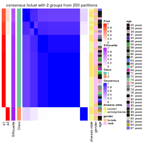
consensus_heatmap(res, k = 3)
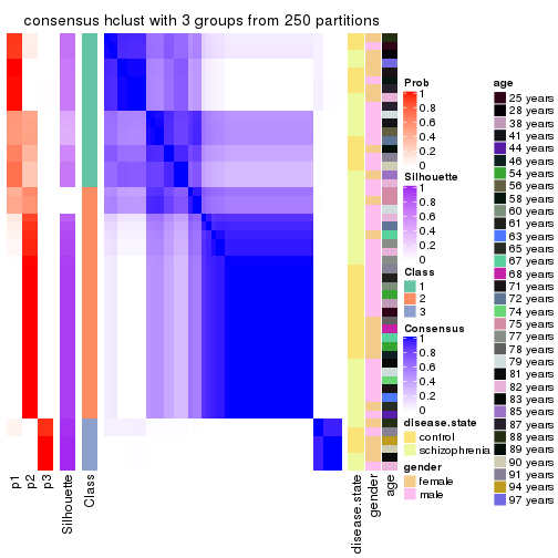
consensus_heatmap(res, k = 4)
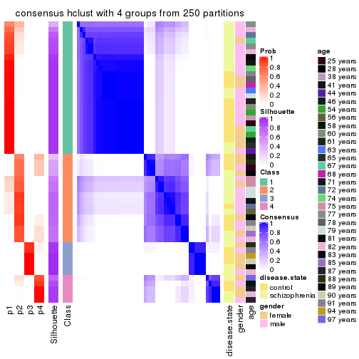
consensus_heatmap(res, k = 5)
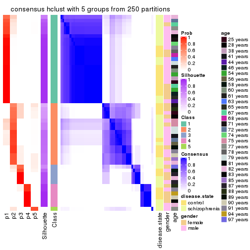
consensus_heatmap(res, k = 6)
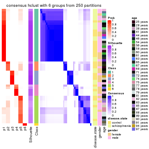
Heatmaps for the membership of samples in all partitions to see how consistent they are:
membership_heatmap(res, k = 2)
membership_heatmap(res, k = 3)
membership_heatmap(res, k = 4)
membership_heatmap(res, k = 5)
membership_heatmap(res, k = 6)
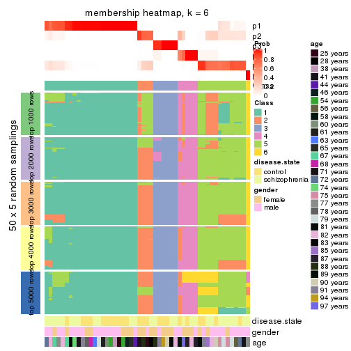
As soon as we have had the classes for columns, we can look for signatures which are significantly different between classes which can be candidate marks for certain classes. Following are the heatmaps for signatures.
Signature heatmaps where rows are scaled:
get_signatures(res, k = 2)
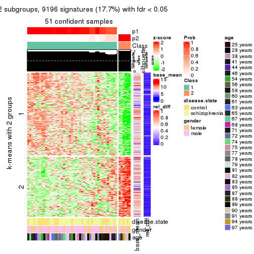
get_signatures(res, k = 3)
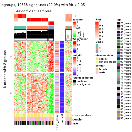
get_signatures(res, k = 4)
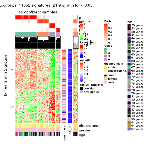
get_signatures(res, k = 5)
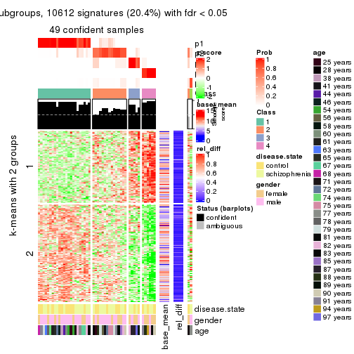
get_signatures(res, k = 6)
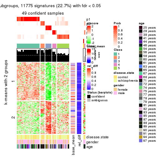
Signature heatmaps where rows are not scaled:
get_signatures(res, k = 2, scale_rows = FALSE)
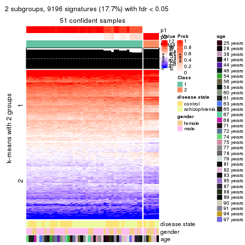
get_signatures(res, k = 3, scale_rows = FALSE)
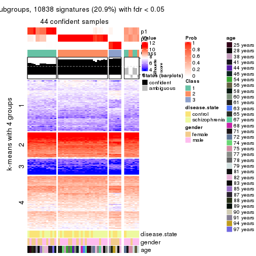
get_signatures(res, k = 4, scale_rows = FALSE)
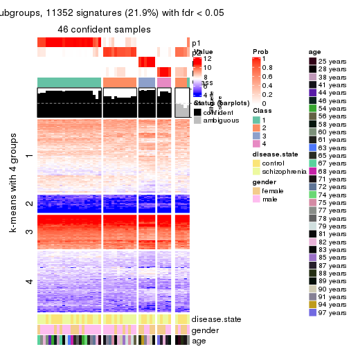
get_signatures(res, k = 5, scale_rows = FALSE)
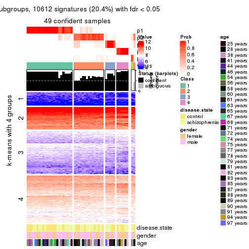
get_signatures(res, k = 6, scale_rows = FALSE)
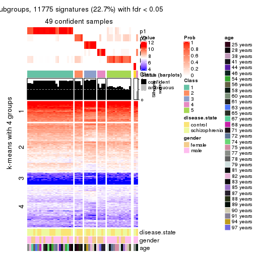
Compare the overlap of signatures from different k:
compare_signatures(res)
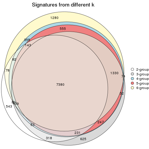
get_signature() returns a data frame invisibly. TO get the list of signatures, the function
call should be assigned to a variable explicitly. In following code, if plot argument is set
to FALSE, no heatmap is plotted while only the differential analysis is performed.
# code only for demonstration
tb = get_signature(res, k = ..., plot = FALSE)
An example of the output of tb is:
#> which_row fdr mean_1 mean_2 scaled_mean_1 scaled_mean_2 km
#> 1 38 0.042760348 8.373488 9.131774 -0.5533452 0.5164555 1
#> 2 40 0.018707592 7.106213 8.469186 -0.6173731 0.5762149 1
#> 3 55 0.019134737 10.221463 11.207825 -0.6159697 0.5749050 1
#> 4 59 0.006059896 5.921854 7.869574 -0.6899429 0.6439467 1
#> 5 60 0.018055526 8.928898 10.211722 -0.6204761 0.5791110 1
#> 6 98 0.009384629 15.714769 14.887706 0.6635654 -0.6193277 2
...
The columns in tb are:
which_row: row indices corresponding to the input matrix.fdr: FDR for the differential test. mean_x: The mean value in group x.scaled_mean_x: The mean value in group x after rows are scaled.km: Row groups if k-means clustering is applied to rows.UMAP plot which shows how samples are separated.
dimension_reduction(res, k = 2, method = "UMAP")
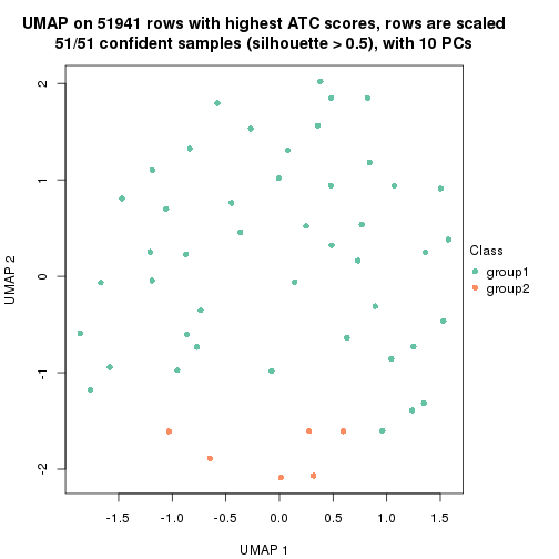
dimension_reduction(res, k = 3, method = "UMAP")
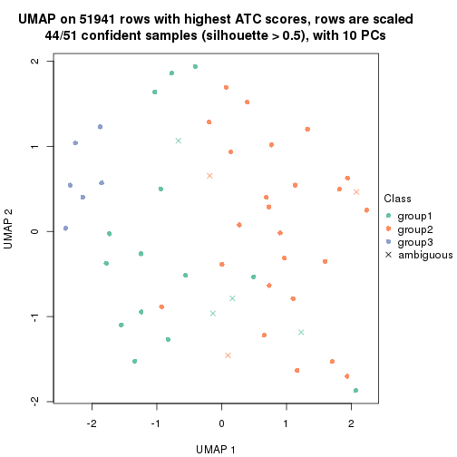
dimension_reduction(res, k = 4, method = "UMAP")
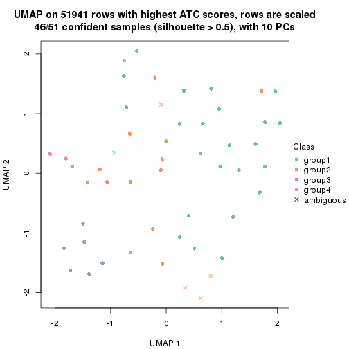
dimension_reduction(res, k = 5, method = "UMAP")
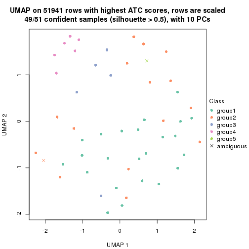
dimension_reduction(res, k = 6, method = "UMAP")
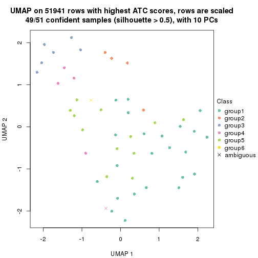
Following heatmap shows how subgroups are split when increasing k:
collect_classes(res)
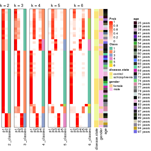
Test correlation between subgroups and known annotations. If the known annotation is numeric, one-way ANOVA test is applied, and if the known annotation is discrete, chi-squared contingency table test is applied.
test_to_known_factors(res)
#> n disease.state(p) gender(p) age(p) k
#> ATC:hclust 51 1.000 0.3072 0.706 2
#> ATC:hclust 44 0.798 0.1118 0.679 3
#> ATC:hclust 46 0.848 0.2062 0.355 4
#> ATC:hclust 49 0.953 0.2867 0.425 5
#> ATC:hclust 49 0.575 0.0992 0.426 6
If matrix rows can be associated to genes, consider to use functional_enrichment(res,
...) to perform function enrichment for the signature genes. See this vignette for more detailed explanations.
The object with results only for a single top-value method and a single partition method can be extracted as:
res = res_list["ATC", "kmeans"]
# you can also extract it by
# res = res_list["ATC:kmeans"]
A summary of res and all the functions that can be applied to it:
res
#> A 'ConsensusPartition' object with k = 2, 3, 4, 5, 6.
#> On a matrix with 51941 rows and 51 columns.
#> Top rows (1000, 2000, 3000, 4000, 5000) are extracted by 'ATC' method.
#> Subgroups are detected by 'kmeans' method.
#> Performed in total 1250 partitions by row resampling.
#> Best k for subgroups seems to be 3.
#>
#> Following methods can be applied to this 'ConsensusPartition' object:
#> [1] "cola_report" "collect_classes" "collect_plots"
#> [4] "collect_stats" "colnames" "compare_signatures"
#> [7] "consensus_heatmap" "dimension_reduction" "functional_enrichment"
#> [10] "get_anno_col" "get_anno" "get_classes"
#> [13] "get_consensus" "get_matrix" "get_membership"
#> [16] "get_param" "get_signatures" "get_stats"
#> [19] "is_best_k" "is_stable_k" "membership_heatmap"
#> [22] "ncol" "nrow" "plot_ecdf"
#> [25] "rownames" "select_partition_number" "show"
#> [28] "suggest_best_k" "test_to_known_factors"
collect_plots() function collects all the plots made from res for all k (number of partitions)
into one single page to provide an easy and fast comparison between different k.
collect_plots(res)
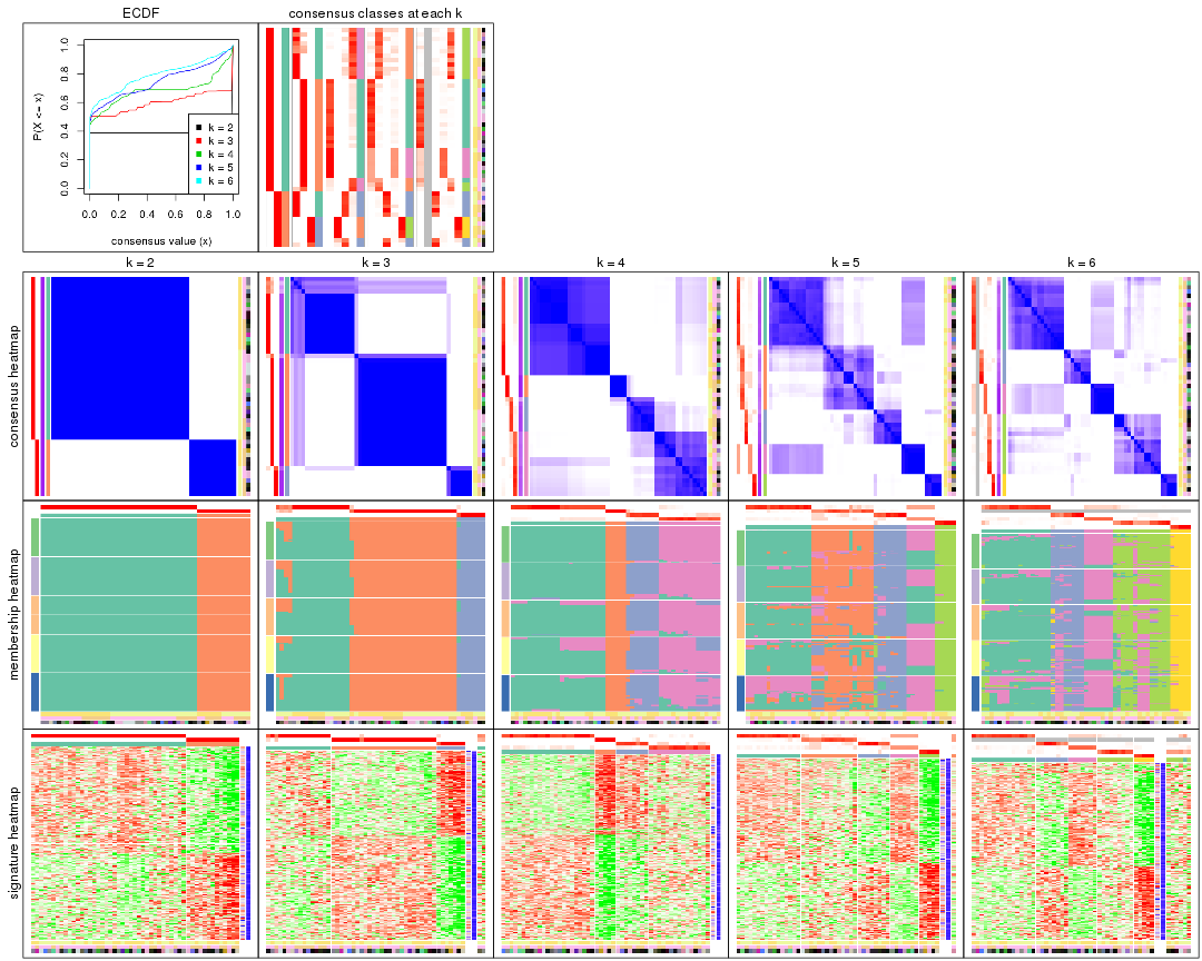
The plots are:
k and the heatmap of
predicted classes for each k.k.k.k.All the plots in panels can be made by individual functions and they are plotted later in this section.
select_partition_number() produces several plots showing different
statistics for choosing “optimized” k. There are following statistics:
k;k, the area increased is defined as \(A_k - A_{k-1}\).The detailed explanations of these statistics can be found in the cola vignette.
Generally speaking, lower PAC score, higher mean silhouette score or higher
concordance corresponds to better partition. Rand index and Jaccard index
measure how similar the current partition is compared to partition with k-1.
If they are too similar, we won't accept k is better than k-1.
select_partition_number(res)
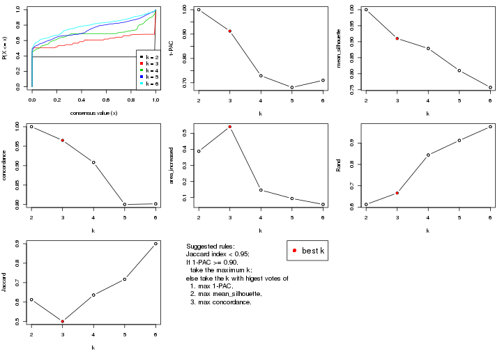
The numeric values for all these statistics can be obtained by get_stats().
get_stats(res)
#> k 1-PAC mean_silhouette concordance area_increased Rand Jaccard
#> 2 2 1.000 1.000 1.000 0.3881 0.613 0.613
#> 3 3 0.912 0.910 0.965 0.5407 0.666 0.501
#> 4 4 0.729 0.879 0.908 0.1465 0.844 0.636
#> 5 5 0.681 0.810 0.800 0.0941 0.912 0.717
#> 6 6 0.710 0.757 0.802 0.0572 0.976 0.900
suggest_best_k() suggests the best \(k\) based on these statistics. The rules are as follows:
suggest_best_k(res)
#> [1] 3
#> attr(,"optional")
#> [1] 2
There is also optional best \(k\) = 2 that is worth to check.
Following shows the table of the partitions (You need to click the show/hide
code output link to see it). The membership matrix (columns with name p*)
is inferred by
clue::cl_consensus()
function with the SE method. Basically the value in the membership matrix
represents the probability to belong to a certain group. The finall class
label for an item is determined with the group with highest probability it
belongs to.
In get_classes() function, the entropy is calculated from the membership
matrix and the silhouette score is calculated from the consensus matrix.
cbind(get_classes(res, k = 2), get_membership(res, k = 2))
#> class entropy silhouette p1 p2
#> GSM439800 1 0 1 1 0
#> GSM439790 1 0 1 1 0
#> GSM439827 1 0 1 1 0
#> GSM439811 1 0 1 1 0
#> GSM439795 2 0 1 0 1
#> GSM439805 2 0 1 0 1
#> GSM439781 1 0 1 1 0
#> GSM439807 2 0 1 0 1
#> GSM439820 2 0 1 0 1
#> GSM439784 1 0 1 1 0
#> GSM439824 1 0 1 1 0
#> GSM439794 1 0 1 1 0
#> GSM439809 1 0 1 1 0
#> GSM439785 1 0 1 1 0
#> GSM439803 1 0 1 1 0
#> GSM439778 1 0 1 1 0
#> GSM439791 1 0 1 1 0
#> GSM439786 1 0 1 1 0
#> GSM439828 1 0 1 1 0
#> GSM439806 1 0 1 1 0
#> GSM439815 1 0 1 1 0
#> GSM439817 1 0 1 1 0
#> GSM439796 1 0 1 1 0
#> GSM439798 2 0 1 0 1
#> GSM439821 2 0 1 0 1
#> GSM439823 1 0 1 1 0
#> GSM439813 1 0 1 1 0
#> GSM439801 2 0 1 0 1
#> GSM439810 1 0 1 1 0
#> GSM439783 1 0 1 1 0
#> GSM439826 1 0 1 1 0
#> GSM439812 1 0 1 1 0
#> GSM439818 2 0 1 0 1
#> GSM439792 1 0 1 1 0
#> GSM439802 2 0 1 0 1
#> GSM439825 1 0 1 1 0
#> GSM439780 1 0 1 1 0
#> GSM439787 2 0 1 0 1
#> GSM439808 2 0 1 0 1
#> GSM439804 1 0 1 1 0
#> GSM439822 1 0 1 1 0
#> GSM439816 1 0 1 1 0
#> GSM439789 1 0 1 1 0
#> GSM439799 2 0 1 0 1
#> GSM439814 1 0 1 1 0
#> GSM439782 1 0 1 1 0
#> GSM439779 1 0 1 1 0
#> GSM439793 1 0 1 1 0
#> GSM439788 1 0 1 1 0
#> GSM439797 1 0 1 1 0
#> GSM439819 2 0 1 0 1
cbind(get_classes(res, k = 3), get_membership(res, k = 3))
#> class entropy silhouette p1 p2 p3
#> GSM439800 1 0.0000 0.890 1.000 0.000 0.000
#> GSM439790 2 0.0000 0.988 0.000 1.000 0.000
#> GSM439827 2 0.0000 0.988 0.000 1.000 0.000
#> GSM439811 1 0.5733 0.568 0.676 0.324 0.000
#> GSM439795 3 0.0000 0.969 0.000 0.000 1.000
#> GSM439805 1 0.0000 0.890 1.000 0.000 0.000
#> GSM439781 1 0.0000 0.890 1.000 0.000 0.000
#> GSM439807 3 0.0000 0.969 0.000 0.000 1.000
#> GSM439820 1 0.0000 0.890 1.000 0.000 0.000
#> GSM439784 1 0.4654 0.693 0.792 0.208 0.000
#> GSM439824 2 0.0000 0.988 0.000 1.000 0.000
#> GSM439794 1 0.6045 0.454 0.620 0.380 0.000
#> GSM439809 2 0.0000 0.988 0.000 1.000 0.000
#> GSM439785 2 0.0000 0.988 0.000 1.000 0.000
#> GSM439803 2 0.0000 0.988 0.000 1.000 0.000
#> GSM439778 2 0.0000 0.988 0.000 1.000 0.000
#> GSM439791 2 0.0000 0.988 0.000 1.000 0.000
#> GSM439786 1 0.6192 0.363 0.580 0.420 0.000
#> GSM439828 2 0.0000 0.988 0.000 1.000 0.000
#> GSM439806 2 0.0000 0.988 0.000 1.000 0.000
#> GSM439815 2 0.0237 0.984 0.004 0.996 0.000
#> GSM439817 1 0.0000 0.890 1.000 0.000 0.000
#> GSM439796 2 0.0000 0.988 0.000 1.000 0.000
#> GSM439798 1 0.0000 0.890 1.000 0.000 0.000
#> GSM439821 3 0.0000 0.969 0.000 0.000 1.000
#> GSM439823 2 0.0000 0.988 0.000 1.000 0.000
#> GSM439813 2 0.0000 0.988 0.000 1.000 0.000
#> GSM439801 3 0.4399 0.781 0.188 0.000 0.812
#> GSM439810 2 0.0000 0.988 0.000 1.000 0.000
#> GSM439783 2 0.0000 0.988 0.000 1.000 0.000
#> GSM439826 2 0.0000 0.988 0.000 1.000 0.000
#> GSM439812 2 0.0000 0.988 0.000 1.000 0.000
#> GSM439818 1 0.0000 0.890 1.000 0.000 0.000
#> GSM439792 2 0.0000 0.988 0.000 1.000 0.000
#> GSM439802 1 0.0000 0.890 1.000 0.000 0.000
#> GSM439825 1 0.0000 0.890 1.000 0.000 0.000
#> GSM439780 1 0.0000 0.890 1.000 0.000 0.000
#> GSM439787 3 0.0000 0.969 0.000 0.000 1.000
#> GSM439808 3 0.0000 0.969 0.000 0.000 1.000
#> GSM439804 2 0.0000 0.988 0.000 1.000 0.000
#> GSM439822 1 0.0000 0.890 1.000 0.000 0.000
#> GSM439816 2 0.0000 0.988 0.000 1.000 0.000
#> GSM439789 2 0.0000 0.988 0.000 1.000 0.000
#> GSM439799 1 0.0000 0.890 1.000 0.000 0.000
#> GSM439814 2 0.0000 0.988 0.000 1.000 0.000
#> GSM439782 2 0.0000 0.988 0.000 1.000 0.000
#> GSM439779 2 0.5254 0.590 0.264 0.736 0.000
#> GSM439793 1 0.0000 0.890 1.000 0.000 0.000
#> GSM439788 1 0.0000 0.890 1.000 0.000 0.000
#> GSM439797 2 0.0000 0.988 0.000 1.000 0.000
#> GSM439819 3 0.0000 0.969 0.000 0.000 1.000
cbind(get_classes(res, k = 4), get_membership(res, k = 4))
#> class entropy silhouette p1 p2 p3 p4
#> GSM439800 4 0.3942 0.743 0.000 0.000 0.236 0.764
#> GSM439790 1 0.1792 0.930 0.932 0.000 0.000 0.068
#> GSM439827 1 0.3266 0.909 0.832 0.000 0.000 0.168
#> GSM439811 4 0.1211 0.829 0.040 0.000 0.000 0.960
#> GSM439795 2 0.0000 1.000 0.000 1.000 0.000 0.000
#> GSM439805 3 0.1792 0.918 0.000 0.000 0.932 0.068
#> GSM439781 4 0.3569 0.764 0.000 0.000 0.196 0.804
#> GSM439807 3 0.4454 0.511 0.000 0.308 0.692 0.000
#> GSM439820 3 0.2281 0.909 0.000 0.000 0.904 0.096
#> GSM439784 4 0.0817 0.833 0.024 0.000 0.000 0.976
#> GSM439824 1 0.0000 0.911 1.000 0.000 0.000 0.000
#> GSM439794 4 0.2048 0.819 0.064 0.000 0.008 0.928
#> GSM439809 1 0.2973 0.927 0.856 0.000 0.000 0.144
#> GSM439785 1 0.2973 0.927 0.856 0.000 0.000 0.144
#> GSM439803 1 0.3123 0.919 0.844 0.000 0.000 0.156
#> GSM439778 1 0.2973 0.927 0.856 0.000 0.000 0.144
#> GSM439791 4 0.3024 0.741 0.148 0.000 0.000 0.852
#> GSM439786 4 0.1792 0.805 0.000 0.000 0.068 0.932
#> GSM439828 1 0.3024 0.925 0.852 0.000 0.000 0.148
#> GSM439806 1 0.1557 0.929 0.944 0.000 0.000 0.056
#> GSM439815 4 0.2868 0.755 0.136 0.000 0.000 0.864
#> GSM439817 4 0.3266 0.777 0.000 0.000 0.168 0.832
#> GSM439796 1 0.3024 0.925 0.852 0.000 0.000 0.148
#> GSM439798 3 0.2469 0.901 0.000 0.000 0.892 0.108
#> GSM439821 2 0.0000 1.000 0.000 1.000 0.000 0.000
#> GSM439823 1 0.3024 0.925 0.852 0.000 0.000 0.148
#> GSM439813 1 0.2814 0.929 0.868 0.000 0.000 0.132
#> GSM439801 3 0.2011 0.855 0.000 0.080 0.920 0.000
#> GSM439810 1 0.0000 0.911 1.000 0.000 0.000 0.000
#> GSM439783 1 0.1557 0.929 0.944 0.000 0.000 0.056
#> GSM439826 1 0.0000 0.911 1.000 0.000 0.000 0.000
#> GSM439812 1 0.1557 0.929 0.944 0.000 0.000 0.056
#> GSM439818 3 0.1940 0.917 0.000 0.000 0.924 0.076
#> GSM439792 1 0.2973 0.927 0.856 0.000 0.000 0.144
#> GSM439802 3 0.1792 0.918 0.000 0.000 0.932 0.068
#> GSM439825 4 0.3907 0.747 0.000 0.000 0.232 0.768
#> GSM439780 4 0.0921 0.834 0.000 0.000 0.028 0.972
#> GSM439787 2 0.0000 1.000 0.000 1.000 0.000 0.000
#> GSM439808 2 0.0000 1.000 0.000 1.000 0.000 0.000
#> GSM439804 1 0.0000 0.911 1.000 0.000 0.000 0.000
#> GSM439822 4 0.3942 0.743 0.000 0.000 0.236 0.764
#> GSM439816 1 0.0000 0.911 1.000 0.000 0.000 0.000
#> GSM439789 1 0.0000 0.911 1.000 0.000 0.000 0.000
#> GSM439799 3 0.1940 0.917 0.000 0.000 0.924 0.076
#> GSM439814 1 0.0000 0.911 1.000 0.000 0.000 0.000
#> GSM439782 1 0.0921 0.921 0.972 0.000 0.000 0.028
#> GSM439779 4 0.1940 0.807 0.076 0.000 0.000 0.924
#> GSM439793 4 0.3569 0.764 0.000 0.000 0.196 0.804
#> GSM439788 4 0.1211 0.832 0.000 0.000 0.040 0.960
#> GSM439797 1 0.2973 0.927 0.856 0.000 0.000 0.144
#> GSM439819 2 0.0000 1.000 0.000 1.000 0.000 0.000
cbind(get_classes(res, k = 5), get_membership(res, k = 5))
#> class entropy silhouette p1 p2 p3 p4 p5
#> GSM439800 2 0.5928 0.551 0.000 0.596 0.192 0.212 0.000
#> GSM439790 1 0.1270 0.837 0.948 0.000 0.000 0.052 0.000
#> GSM439827 1 0.4088 0.663 0.776 0.168 0.000 0.056 0.000
#> GSM439811 2 0.3291 0.735 0.120 0.840 0.000 0.040 0.000
#> GSM439795 5 0.0000 0.986 0.000 0.000 0.000 0.000 1.000
#> GSM439805 3 0.0000 0.883 0.000 0.000 1.000 0.000 0.000
#> GSM439781 2 0.3476 0.688 0.000 0.804 0.176 0.020 0.000
#> GSM439807 3 0.4042 0.634 0.000 0.000 0.756 0.032 0.212
#> GSM439820 3 0.1251 0.873 0.000 0.036 0.956 0.008 0.000
#> GSM439784 2 0.2595 0.747 0.080 0.888 0.000 0.032 0.000
#> GSM439824 4 0.4283 0.992 0.456 0.000 0.000 0.544 0.000
#> GSM439794 2 0.5268 0.702 0.168 0.692 0.004 0.136 0.000
#> GSM439809 1 0.1893 0.864 0.928 0.048 0.000 0.024 0.000
#> GSM439785 1 0.0404 0.869 0.988 0.000 0.000 0.012 0.000
#> GSM439803 1 0.1943 0.832 0.924 0.020 0.000 0.056 0.000
#> GSM439778 1 0.0955 0.864 0.968 0.004 0.000 0.028 0.000
#> GSM439791 2 0.5177 0.124 0.472 0.488 0.000 0.040 0.000
#> GSM439786 2 0.4613 0.639 0.072 0.728 0.000 0.200 0.000
#> GSM439828 1 0.1800 0.866 0.932 0.048 0.000 0.020 0.000
#> GSM439806 1 0.2903 0.808 0.872 0.048 0.000 0.080 0.000
#> GSM439815 2 0.4844 0.612 0.280 0.668 0.000 0.052 0.000
#> GSM439817 2 0.2616 0.715 0.000 0.880 0.100 0.020 0.000
#> GSM439796 1 0.1557 0.847 0.940 0.008 0.000 0.052 0.000
#> GSM439798 3 0.1914 0.856 0.000 0.060 0.924 0.016 0.000
#> GSM439821 5 0.0000 0.986 0.000 0.000 0.000 0.000 1.000
#> GSM439823 1 0.0703 0.870 0.976 0.000 0.000 0.024 0.000
#> GSM439813 1 0.2514 0.849 0.896 0.044 0.000 0.060 0.000
#> GSM439801 3 0.0510 0.879 0.000 0.000 0.984 0.000 0.016
#> GSM439810 4 0.4283 0.992 0.456 0.000 0.000 0.544 0.000
#> GSM439783 1 0.1121 0.842 0.956 0.000 0.000 0.044 0.000
#> GSM439826 4 0.4283 0.992 0.456 0.000 0.000 0.544 0.000
#> GSM439812 1 0.2903 0.808 0.872 0.048 0.000 0.080 0.000
#> GSM439818 3 0.3991 0.777 0.000 0.048 0.780 0.172 0.000
#> GSM439792 1 0.2149 0.859 0.916 0.048 0.000 0.036 0.000
#> GSM439802 3 0.0000 0.883 0.000 0.000 1.000 0.000 0.000
#> GSM439825 2 0.5997 0.560 0.004 0.604 0.188 0.204 0.000
#> GSM439780 2 0.2812 0.746 0.096 0.876 0.024 0.004 0.000
#> GSM439787 5 0.0000 0.986 0.000 0.000 0.000 0.000 1.000
#> GSM439808 5 0.0880 0.979 0.000 0.000 0.000 0.032 0.968
#> GSM439804 4 0.4294 0.962 0.468 0.000 0.000 0.532 0.000
#> GSM439822 2 0.5928 0.551 0.000 0.596 0.192 0.212 0.000
#> GSM439816 4 0.4283 0.992 0.456 0.000 0.000 0.544 0.000
#> GSM439789 4 0.4278 0.987 0.452 0.000 0.000 0.548 0.000
#> GSM439799 3 0.3495 0.800 0.000 0.032 0.816 0.152 0.000
#> GSM439814 4 0.4283 0.992 0.456 0.000 0.000 0.544 0.000
#> GSM439782 1 0.1544 0.812 0.932 0.000 0.000 0.068 0.000
#> GSM439779 2 0.3412 0.727 0.152 0.820 0.000 0.028 0.000
#> GSM439793 2 0.3476 0.688 0.000 0.804 0.176 0.020 0.000
#> GSM439788 2 0.2142 0.749 0.048 0.920 0.028 0.004 0.000
#> GSM439797 1 0.1124 0.875 0.960 0.036 0.000 0.004 0.000
#> GSM439819 5 0.1281 0.973 0.000 0.000 0.012 0.032 0.956
cbind(get_classes(res, k = 6), get_membership(res, k = 6))
#> class entropy silhouette p1 p2 p3 p4 p5 p6
#> GSM439800 5 0.4847 0.476 0.000 NA 0.056 0.000 0.500 0.000
#> GSM439790 1 0.1616 0.819 0.932 NA 0.000 0.020 0.000 0.000
#> GSM439827 1 0.5209 0.635 0.680 NA 0.000 0.048 0.184 0.000
#> GSM439811 5 0.3553 0.681 0.068 NA 0.000 0.016 0.820 0.000
#> GSM439795 6 0.0000 0.965 0.000 NA 0.000 0.000 0.000 1.000
#> GSM439805 3 0.0000 0.806 0.000 NA 1.000 0.000 0.000 0.000
#> GSM439781 5 0.3865 0.640 0.000 NA 0.072 0.040 0.808 0.000
#> GSM439807 3 0.4364 0.661 0.000 NA 0.764 0.060 0.004 0.140
#> GSM439820 3 0.3407 0.770 0.000 NA 0.840 0.040 0.048 0.000
#> GSM439784 5 0.2226 0.714 0.028 NA 0.000 0.008 0.904 0.000
#> GSM439824 4 0.3023 0.990 0.232 NA 0.000 0.768 0.000 0.000
#> GSM439794 5 0.5750 0.588 0.172 NA 0.000 0.020 0.584 0.000
#> GSM439809 1 0.2673 0.793 0.880 NA 0.000 0.044 0.012 0.000
#> GSM439785 1 0.1434 0.822 0.940 NA 0.000 0.012 0.000 0.000
#> GSM439803 1 0.3048 0.788 0.860 NA 0.000 0.024 0.044 0.000
#> GSM439778 1 0.2113 0.817 0.908 NA 0.000 0.028 0.004 0.000
#> GSM439791 1 0.5691 0.222 0.504 NA 0.000 0.016 0.372 0.000
#> GSM439786 5 0.5899 0.400 0.024 NA 0.000 0.112 0.468 0.000
#> GSM439828 1 0.0964 0.828 0.968 NA 0.000 0.004 0.016 0.000
#> GSM439806 1 0.3677 0.729 0.804 NA 0.000 0.120 0.012 0.000
#> GSM439815 5 0.5722 0.440 0.300 NA 0.000 0.024 0.560 0.000
#> GSM439817 5 0.1624 0.707 0.004 NA 0.000 0.020 0.936 0.000
#> GSM439796 1 0.2594 0.809 0.884 NA 0.000 0.028 0.016 0.000
#> GSM439798 3 0.3702 0.759 0.000 NA 0.820 0.040 0.064 0.000
#> GSM439821 6 0.0000 0.965 0.000 NA 0.000 0.000 0.000 1.000
#> GSM439823 1 0.1801 0.825 0.924 NA 0.000 0.016 0.004 0.000
#> GSM439813 1 0.4083 0.735 0.780 NA 0.000 0.124 0.024 0.000
#> GSM439801 3 0.0725 0.803 0.000 NA 0.976 0.012 0.000 0.000
#> GSM439810 4 0.3023 0.990 0.232 NA 0.000 0.768 0.000 0.000
#> GSM439783 1 0.1616 0.819 0.932 NA 0.000 0.020 0.000 0.000
#> GSM439826 4 0.3163 0.987 0.232 NA 0.000 0.764 0.000 0.000
#> GSM439812 1 0.3677 0.729 0.804 NA 0.000 0.120 0.012 0.000
#> GSM439818 3 0.4549 0.553 0.000 NA 0.552 0.004 0.028 0.000
#> GSM439792 1 0.2889 0.794 0.868 NA 0.000 0.048 0.016 0.000
#> GSM439802 3 0.0146 0.806 0.000 NA 0.996 0.000 0.000 0.000
#> GSM439825 5 0.4844 0.478 0.000 NA 0.056 0.000 0.504 0.000
#> GSM439780 5 0.1003 0.715 0.020 NA 0.000 0.000 0.964 0.000
#> GSM439787 6 0.0000 0.965 0.000 NA 0.000 0.000 0.000 1.000
#> GSM439808 6 0.1844 0.947 0.000 NA 0.000 0.048 0.004 0.924
#> GSM439804 4 0.3244 0.945 0.268 NA 0.000 0.732 0.000 0.000
#> GSM439822 5 0.4847 0.476 0.000 NA 0.056 0.000 0.500 0.000
#> GSM439816 4 0.3023 0.990 0.232 NA 0.000 0.768 0.000 0.000
#> GSM439789 4 0.3023 0.990 0.232 NA 0.000 0.768 0.000 0.000
#> GSM439799 3 0.3898 0.621 0.000 NA 0.652 0.000 0.012 0.000
#> GSM439814 4 0.3023 0.990 0.232 NA 0.000 0.768 0.000 0.000
#> GSM439782 1 0.1700 0.816 0.928 NA 0.000 0.024 0.000 0.000
#> GSM439779 5 0.3357 0.694 0.064 NA 0.000 0.012 0.832 0.000
#> GSM439793 5 0.3865 0.640 0.000 NA 0.072 0.040 0.808 0.000
#> GSM439788 5 0.0405 0.715 0.008 NA 0.000 0.000 0.988 0.000
#> GSM439797 1 0.0665 0.827 0.980 NA 0.000 0.008 0.004 0.000
#> GSM439819 6 0.2445 0.932 0.000 NA 0.008 0.060 0.004 0.896
Heatmaps for the consensus matrix. It visualizes the probability of two samples to be in a same group.
consensus_heatmap(res, k = 2)
consensus_heatmap(res, k = 3)
consensus_heatmap(res, k = 4)
consensus_heatmap(res, k = 5)
consensus_heatmap(res, k = 6)
Heatmaps for the membership of samples in all partitions to see how consistent they are:
membership_heatmap(res, k = 2)
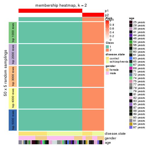
membership_heatmap(res, k = 3)
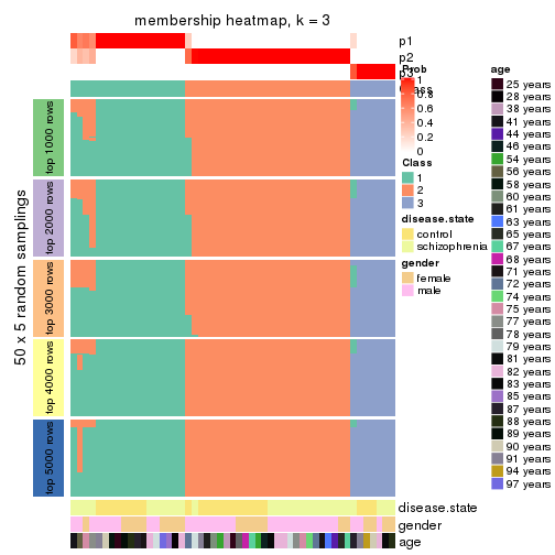
membership_heatmap(res, k = 4)
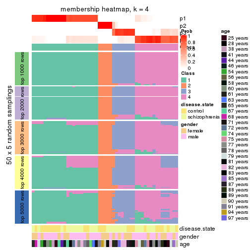
membership_heatmap(res, k = 5)
membership_heatmap(res, k = 6)
As soon as we have had the classes for columns, we can look for signatures which are significantly different between classes which can be candidate marks for certain classes. Following are the heatmaps for signatures.
Signature heatmaps where rows are scaled:
get_signatures(res, k = 2)
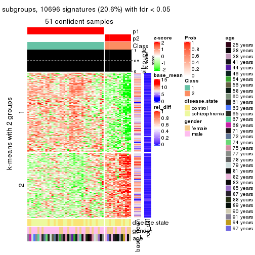
get_signatures(res, k = 3)
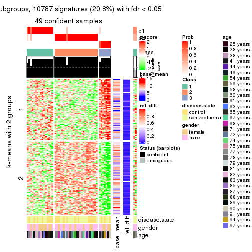
get_signatures(res, k = 4)
get_signatures(res, k = 5)
get_signatures(res, k = 6)
Signature heatmaps where rows are not scaled:
get_signatures(res, k = 2, scale_rows = FALSE)
get_signatures(res, k = 3, scale_rows = FALSE)
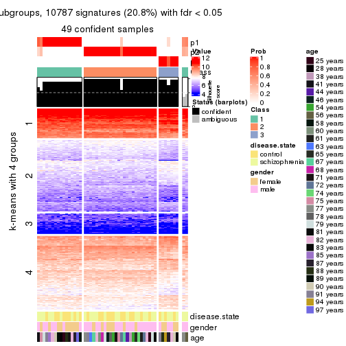
get_signatures(res, k = 4, scale_rows = FALSE)
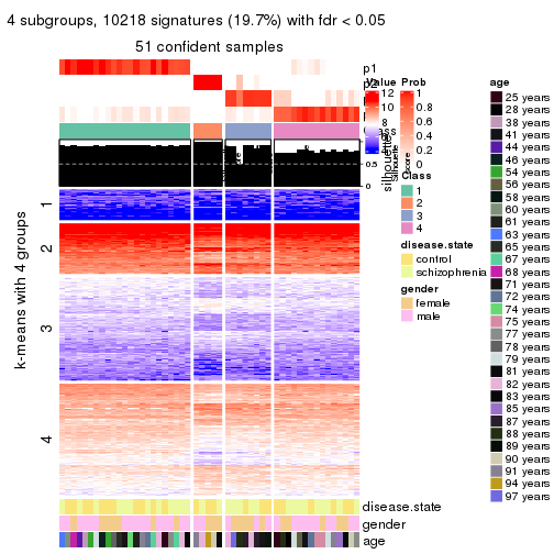
get_signatures(res, k = 5, scale_rows = FALSE)
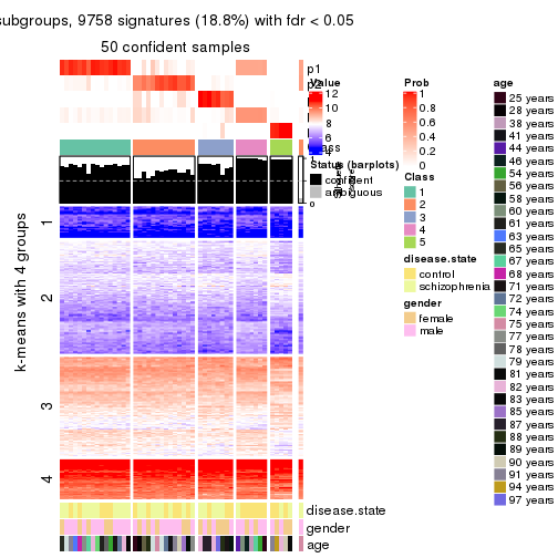
get_signatures(res, k = 6, scale_rows = FALSE)
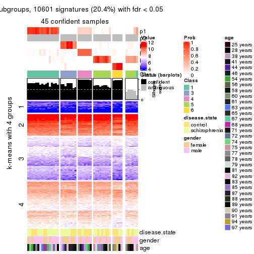
Compare the overlap of signatures from different k:
compare_signatures(res)
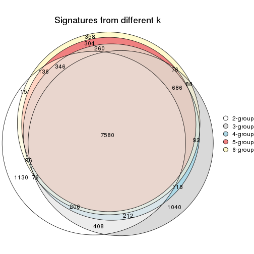
get_signature() returns a data frame invisibly. TO get the list of signatures, the function
call should be assigned to a variable explicitly. In following code, if plot argument is set
to FALSE, no heatmap is plotted while only the differential analysis is performed.
# code only for demonstration
tb = get_signature(res, k = ..., plot = FALSE)
An example of the output of tb is:
#> which_row fdr mean_1 mean_2 scaled_mean_1 scaled_mean_2 km
#> 1 38 0.042760348 8.373488 9.131774 -0.5533452 0.5164555 1
#> 2 40 0.018707592 7.106213 8.469186 -0.6173731 0.5762149 1
#> 3 55 0.019134737 10.221463 11.207825 -0.6159697 0.5749050 1
#> 4 59 0.006059896 5.921854 7.869574 -0.6899429 0.6439467 1
#> 5 60 0.018055526 8.928898 10.211722 -0.6204761 0.5791110 1
#> 6 98 0.009384629 15.714769 14.887706 0.6635654 -0.6193277 2
...
The columns in tb are:
which_row: row indices corresponding to the input matrix.fdr: FDR for the differential test. mean_x: The mean value in group x.scaled_mean_x: The mean value in group x after rows are scaled.km: Row groups if k-means clustering is applied to rows.UMAP plot which shows how samples are separated.
dimension_reduction(res, k = 2, method = "UMAP")
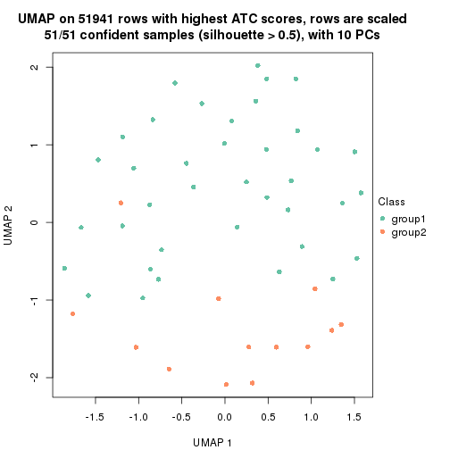
dimension_reduction(res, k = 3, method = "UMAP")
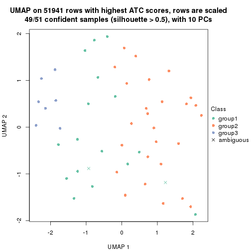
dimension_reduction(res, k = 4, method = "UMAP")
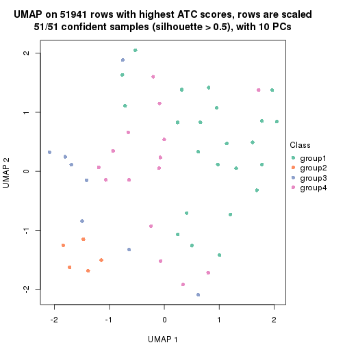
dimension_reduction(res, k = 5, method = "UMAP")
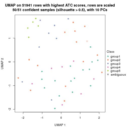
dimension_reduction(res, k = 6, method = "UMAP")
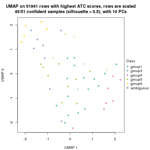
Following heatmap shows how subgroups are split when increasing k:
collect_classes(res)
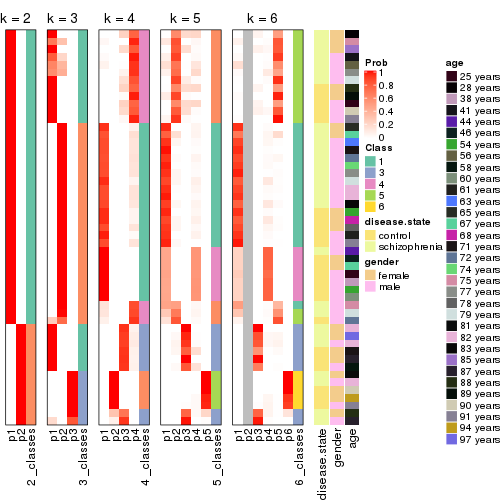
Test correlation between subgroups and known annotations. If the known annotation is numeric, one-way ANOVA test is applied, and if the known annotation is discrete, chi-squared contingency table test is applied.
test_to_known_factors(res)
#> n disease.state(p) gender(p) age(p) k
#> ATC:kmeans 51 1.000 0.114 0.405 2
#> ATC:kmeans 49 0.945 0.109 0.794 3
#> ATC:kmeans 51 0.835 0.297 0.486 4
#> ATC:kmeans 50 0.163 0.475 0.522 5
#> ATC:kmeans 45 0.167 0.466 0.504 6
If matrix rows can be associated to genes, consider to use functional_enrichment(res,
...) to perform function enrichment for the signature genes. See this vignette for more detailed explanations.
The object with results only for a single top-value method and a single partition method can be extracted as:
res = res_list["ATC", "skmeans"]
# you can also extract it by
# res = res_list["ATC:skmeans"]
A summary of res and all the functions that can be applied to it:
res
#> A 'ConsensusPartition' object with k = 2, 3, 4, 5, 6.
#> On a matrix with 51941 rows and 51 columns.
#> Top rows (1000, 2000, 3000, 4000, 5000) are extracted by 'ATC' method.
#> Subgroups are detected by 'skmeans' method.
#> Performed in total 1250 partitions by row resampling.
#> Best k for subgroups seems to be 2.
#>
#> Following methods can be applied to this 'ConsensusPartition' object:
#> [1] "cola_report" "collect_classes" "collect_plots"
#> [4] "collect_stats" "colnames" "compare_signatures"
#> [7] "consensus_heatmap" "dimension_reduction" "functional_enrichment"
#> [10] "get_anno_col" "get_anno" "get_classes"
#> [13] "get_consensus" "get_matrix" "get_membership"
#> [16] "get_param" "get_signatures" "get_stats"
#> [19] "is_best_k" "is_stable_k" "membership_heatmap"
#> [22] "ncol" "nrow" "plot_ecdf"
#> [25] "rownames" "select_partition_number" "show"
#> [28] "suggest_best_k" "test_to_known_factors"
collect_plots() function collects all the plots made from res for all k (number of partitions)
into one single page to provide an easy and fast comparison between different k.
collect_plots(res)
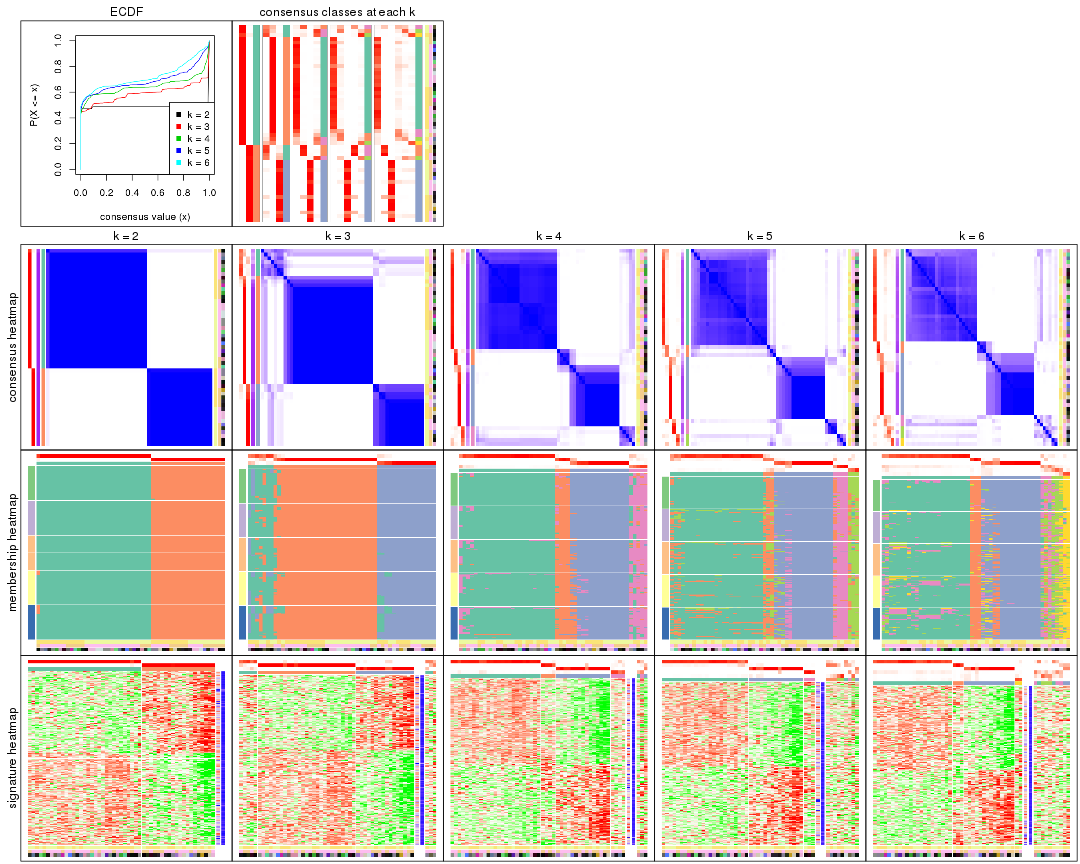
The plots are:
k and the heatmap of
predicted classes for each k.k.k.k.All the plots in panels can be made by individual functions and they are plotted later in this section.
select_partition_number() produces several plots showing different
statistics for choosing “optimized” k. There are following statistics:
k;k, the area increased is defined as \(A_k - A_{k-1}\).The detailed explanations of these statistics can be found in the cola vignette.
Generally speaking, lower PAC score, higher mean silhouette score or higher
concordance corresponds to better partition. Rand index and Jaccard index
measure how similar the current partition is compared to partition with k-1.
If they are too similar, we won't accept k is better than k-1.
select_partition_number(res)
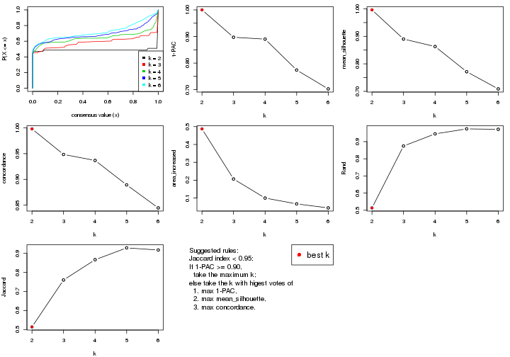
The numeric values for all these statistics can be obtained by get_stats().
get_stats(res)
#> k 1-PAC mean_silhouette concordance area_increased Rand Jaccard
#> 2 2 1.000 0.996 0.998 0.4874 0.514 0.514
#> 3 3 0.897 0.890 0.948 0.2068 0.875 0.760
#> 4 4 0.890 0.863 0.937 0.0999 0.945 0.867
#> 5 5 0.774 0.771 0.889 0.0672 0.974 0.929
#> 6 6 0.703 0.709 0.844 0.0448 0.972 0.918
suggest_best_k() suggests the best \(k\) based on these statistics. The rules are as follows:
suggest_best_k(res)
#> [1] 2
Following shows the table of the partitions (You need to click the show/hide
code output link to see it). The membership matrix (columns with name p*)
is inferred by
clue::cl_consensus()
function with the SE method. Basically the value in the membership matrix
represents the probability to belong to a certain group. The finall class
label for an item is determined with the group with highest probability it
belongs to.
In get_classes() function, the entropy is calculated from the membership
matrix and the silhouette score is calculated from the consensus matrix.
cbind(get_classes(res, k = 2), get_membership(res, k = 2))
#> class entropy silhouette p1 p2
#> GSM439800 2 0.0000 1.000 0.000 1.000
#> GSM439790 1 0.0000 0.997 1.000 0.000
#> GSM439827 1 0.0000 0.997 1.000 0.000
#> GSM439811 1 0.0000 0.997 1.000 0.000
#> GSM439795 2 0.0000 1.000 0.000 1.000
#> GSM439805 2 0.0000 1.000 0.000 1.000
#> GSM439781 2 0.0000 1.000 0.000 1.000
#> GSM439807 2 0.0000 1.000 0.000 1.000
#> GSM439820 2 0.0000 1.000 0.000 1.000
#> GSM439784 1 0.0000 0.997 1.000 0.000
#> GSM439824 1 0.0000 0.997 1.000 0.000
#> GSM439794 1 0.0000 0.997 1.000 0.000
#> GSM439809 1 0.0000 0.997 1.000 0.000
#> GSM439785 1 0.0000 0.997 1.000 0.000
#> GSM439803 1 0.0000 0.997 1.000 0.000
#> GSM439778 1 0.0000 0.997 1.000 0.000
#> GSM439791 1 0.0000 0.997 1.000 0.000
#> GSM439786 1 0.0000 0.997 1.000 0.000
#> GSM439828 1 0.0000 0.997 1.000 0.000
#> GSM439806 1 0.0000 0.997 1.000 0.000
#> GSM439815 1 0.0000 0.997 1.000 0.000
#> GSM439817 2 0.0000 1.000 0.000 1.000
#> GSM439796 1 0.0000 0.997 1.000 0.000
#> GSM439798 2 0.0000 1.000 0.000 1.000
#> GSM439821 2 0.0000 1.000 0.000 1.000
#> GSM439823 1 0.0000 0.997 1.000 0.000
#> GSM439813 1 0.0000 0.997 1.000 0.000
#> GSM439801 2 0.0000 1.000 0.000 1.000
#> GSM439810 1 0.0000 0.997 1.000 0.000
#> GSM439783 1 0.0000 0.997 1.000 0.000
#> GSM439826 1 0.0000 0.997 1.000 0.000
#> GSM439812 1 0.0000 0.997 1.000 0.000
#> GSM439818 2 0.0000 1.000 0.000 1.000
#> GSM439792 1 0.0000 0.997 1.000 0.000
#> GSM439802 2 0.0000 1.000 0.000 1.000
#> GSM439825 2 0.0000 1.000 0.000 1.000
#> GSM439780 1 0.4161 0.908 0.916 0.084
#> GSM439787 2 0.0000 1.000 0.000 1.000
#> GSM439808 2 0.0000 1.000 0.000 1.000
#> GSM439804 1 0.0000 0.997 1.000 0.000
#> GSM439822 2 0.0000 1.000 0.000 1.000
#> GSM439816 1 0.0000 0.997 1.000 0.000
#> GSM439789 1 0.0000 0.997 1.000 0.000
#> GSM439799 2 0.0000 1.000 0.000 1.000
#> GSM439814 1 0.0000 0.997 1.000 0.000
#> GSM439782 1 0.0000 0.997 1.000 0.000
#> GSM439779 1 0.0000 0.997 1.000 0.000
#> GSM439793 2 0.0000 1.000 0.000 1.000
#> GSM439788 2 0.0672 0.992 0.008 0.992
#> GSM439797 1 0.0000 0.997 1.000 0.000
#> GSM439819 2 0.0000 1.000 0.000 1.000
cbind(get_classes(res, k = 3), get_membership(res, k = 3))
#> class entropy silhouette p1 p2 p3
#> GSM439800 1 0.2878 0.702 0.904 0.000 0.096
#> GSM439790 2 0.0000 0.976 0.000 1.000 0.000
#> GSM439827 2 0.0000 0.976 0.000 1.000 0.000
#> GSM439811 2 0.2165 0.910 0.064 0.936 0.000
#> GSM439795 3 0.0000 0.959 0.000 0.000 1.000
#> GSM439805 3 0.0000 0.959 0.000 0.000 1.000
#> GSM439781 3 0.2165 0.902 0.064 0.000 0.936
#> GSM439807 3 0.0000 0.959 0.000 0.000 1.000
#> GSM439820 3 0.0000 0.959 0.000 0.000 1.000
#> GSM439784 1 0.5178 0.613 0.744 0.256 0.000
#> GSM439824 2 0.0000 0.976 0.000 1.000 0.000
#> GSM439794 1 0.5948 0.445 0.640 0.360 0.000
#> GSM439809 2 0.0000 0.976 0.000 1.000 0.000
#> GSM439785 2 0.0000 0.976 0.000 1.000 0.000
#> GSM439803 2 0.0000 0.976 0.000 1.000 0.000
#> GSM439778 2 0.0000 0.976 0.000 1.000 0.000
#> GSM439791 2 0.0000 0.976 0.000 1.000 0.000
#> GSM439786 2 0.5988 0.347 0.368 0.632 0.000
#> GSM439828 2 0.0000 0.976 0.000 1.000 0.000
#> GSM439806 2 0.0000 0.976 0.000 1.000 0.000
#> GSM439815 2 0.0000 0.976 0.000 1.000 0.000
#> GSM439817 3 0.0237 0.956 0.004 0.000 0.996
#> GSM439796 2 0.0000 0.976 0.000 1.000 0.000
#> GSM439798 3 0.0000 0.959 0.000 0.000 1.000
#> GSM439821 3 0.0000 0.959 0.000 0.000 1.000
#> GSM439823 2 0.0000 0.976 0.000 1.000 0.000
#> GSM439813 2 0.0000 0.976 0.000 1.000 0.000
#> GSM439801 3 0.0000 0.959 0.000 0.000 1.000
#> GSM439810 2 0.0000 0.976 0.000 1.000 0.000
#> GSM439783 2 0.0000 0.976 0.000 1.000 0.000
#> GSM439826 2 0.0000 0.976 0.000 1.000 0.000
#> GSM439812 2 0.0000 0.976 0.000 1.000 0.000
#> GSM439818 3 0.4291 0.764 0.180 0.000 0.820
#> GSM439792 2 0.0000 0.976 0.000 1.000 0.000
#> GSM439802 3 0.0000 0.959 0.000 0.000 1.000
#> GSM439825 1 0.2356 0.707 0.928 0.000 0.072
#> GSM439780 1 0.4232 0.712 0.872 0.084 0.044
#> GSM439787 3 0.0000 0.959 0.000 0.000 1.000
#> GSM439808 3 0.0000 0.959 0.000 0.000 1.000
#> GSM439804 2 0.0000 0.976 0.000 1.000 0.000
#> GSM439822 1 0.5397 0.527 0.720 0.000 0.280
#> GSM439816 2 0.0000 0.976 0.000 1.000 0.000
#> GSM439789 2 0.0000 0.976 0.000 1.000 0.000
#> GSM439799 3 0.4452 0.747 0.192 0.000 0.808
#> GSM439814 2 0.0000 0.976 0.000 1.000 0.000
#> GSM439782 2 0.0000 0.976 0.000 1.000 0.000
#> GSM439779 2 0.3752 0.810 0.144 0.856 0.000
#> GSM439793 3 0.2356 0.893 0.072 0.000 0.928
#> GSM439788 1 0.5882 0.412 0.652 0.000 0.348
#> GSM439797 2 0.0000 0.976 0.000 1.000 0.000
#> GSM439819 3 0.0000 0.959 0.000 0.000 1.000
cbind(get_classes(res, k = 4), get_membership(res, k = 4))
#> class entropy silhouette p1 p2 p3 p4
#> GSM439800 2 0.0336 0.901 0.000 0.992 0.008 0.000
#> GSM439790 1 0.0657 0.951 0.984 0.004 0.000 0.012
#> GSM439827 1 0.2466 0.881 0.900 0.004 0.000 0.096
#> GSM439811 1 0.5112 0.302 0.608 0.008 0.000 0.384
#> GSM439795 3 0.0000 0.942 0.000 0.000 1.000 0.000
#> GSM439805 3 0.0000 0.942 0.000 0.000 1.000 0.000
#> GSM439781 3 0.1302 0.917 0.000 0.000 0.956 0.044
#> GSM439807 3 0.0000 0.942 0.000 0.000 1.000 0.000
#> GSM439820 3 0.0000 0.942 0.000 0.000 1.000 0.000
#> GSM439784 4 0.2660 0.601 0.036 0.056 0.000 0.908
#> GSM439824 1 0.0000 0.953 1.000 0.000 0.000 0.000
#> GSM439794 2 0.4635 0.719 0.080 0.796 0.000 0.124
#> GSM439809 1 0.0707 0.948 0.980 0.000 0.000 0.020
#> GSM439785 1 0.0657 0.951 0.984 0.004 0.000 0.012
#> GSM439803 1 0.1004 0.945 0.972 0.004 0.000 0.024
#> GSM439778 1 0.0779 0.950 0.980 0.004 0.000 0.016
#> GSM439791 1 0.2973 0.824 0.856 0.000 0.000 0.144
#> GSM439786 4 0.6221 0.462 0.316 0.076 0.000 0.608
#> GSM439828 1 0.0707 0.949 0.980 0.000 0.000 0.020
#> GSM439806 1 0.0707 0.948 0.980 0.000 0.000 0.020
#> GSM439815 1 0.2988 0.849 0.876 0.012 0.000 0.112
#> GSM439817 3 0.1767 0.910 0.000 0.012 0.944 0.044
#> GSM439796 1 0.0804 0.949 0.980 0.008 0.000 0.012
#> GSM439798 3 0.0000 0.942 0.000 0.000 1.000 0.000
#> GSM439821 3 0.0000 0.942 0.000 0.000 1.000 0.000
#> GSM439823 1 0.0779 0.950 0.980 0.004 0.000 0.016
#> GSM439813 1 0.0336 0.952 0.992 0.000 0.000 0.008
#> GSM439801 3 0.0000 0.942 0.000 0.000 1.000 0.000
#> GSM439810 1 0.0000 0.953 1.000 0.000 0.000 0.000
#> GSM439783 1 0.0524 0.952 0.988 0.004 0.000 0.008
#> GSM439826 1 0.0000 0.953 1.000 0.000 0.000 0.000
#> GSM439812 1 0.0707 0.948 0.980 0.000 0.000 0.020
#> GSM439818 3 0.4477 0.568 0.000 0.312 0.688 0.000
#> GSM439792 1 0.0592 0.950 0.984 0.000 0.000 0.016
#> GSM439802 3 0.0000 0.942 0.000 0.000 1.000 0.000
#> GSM439825 2 0.0895 0.896 0.000 0.976 0.004 0.020
#> GSM439780 4 0.4478 0.572 0.048 0.132 0.008 0.812
#> GSM439787 3 0.0000 0.942 0.000 0.000 1.000 0.000
#> GSM439808 3 0.0000 0.942 0.000 0.000 1.000 0.000
#> GSM439804 1 0.0657 0.951 0.984 0.004 0.000 0.012
#> GSM439822 2 0.1004 0.893 0.000 0.972 0.024 0.004
#> GSM439816 1 0.0000 0.953 1.000 0.000 0.000 0.000
#> GSM439789 1 0.0524 0.952 0.988 0.004 0.000 0.008
#> GSM439799 3 0.4746 0.454 0.000 0.368 0.632 0.000
#> GSM439814 1 0.0592 0.950 0.984 0.000 0.000 0.016
#> GSM439782 1 0.0657 0.951 0.984 0.004 0.000 0.012
#> GSM439779 4 0.4744 0.503 0.284 0.012 0.000 0.704
#> GSM439793 3 0.1474 0.912 0.000 0.000 0.948 0.052
#> GSM439788 4 0.2675 0.574 0.000 0.044 0.048 0.908
#> GSM439797 1 0.0469 0.951 0.988 0.000 0.000 0.012
#> GSM439819 3 0.0000 0.942 0.000 0.000 1.000 0.000
cbind(get_classes(res, k = 5), get_membership(res, k = 5))
#> class entropy silhouette p1 p2 p3 p4 p5
#> GSM439800 4 0.0613 0.8182 0.000 0.008 0.004 0.984 0.004
#> GSM439790 1 0.1399 0.8940 0.952 0.028 0.000 0.000 0.020
#> GSM439827 1 0.3807 0.6674 0.748 0.240 0.000 0.000 0.012
#> GSM439811 2 0.4665 0.3283 0.260 0.692 0.000 0.000 0.048
#> GSM439795 3 0.0000 0.9165 0.000 0.000 1.000 0.000 0.000
#> GSM439805 3 0.0000 0.9165 0.000 0.000 1.000 0.000 0.000
#> GSM439781 3 0.2984 0.8276 0.000 0.032 0.860 0.000 0.108
#> GSM439807 3 0.0000 0.9165 0.000 0.000 1.000 0.000 0.000
#> GSM439820 3 0.0000 0.9165 0.000 0.000 1.000 0.000 0.000
#> GSM439784 2 0.4869 0.0953 0.016 0.656 0.000 0.020 0.308
#> GSM439824 1 0.0510 0.8990 0.984 0.016 0.000 0.000 0.000
#> GSM439794 4 0.5889 0.3513 0.044 0.384 0.000 0.540 0.032
#> GSM439809 1 0.1341 0.8883 0.944 0.056 0.000 0.000 0.000
#> GSM439785 1 0.1364 0.8941 0.952 0.036 0.000 0.000 0.012
#> GSM439803 1 0.2450 0.8659 0.896 0.076 0.000 0.000 0.028
#> GSM439778 1 0.2331 0.8687 0.900 0.080 0.000 0.000 0.020
#> GSM439791 1 0.4713 0.5118 0.676 0.280 0.000 0.000 0.044
#> GSM439786 5 0.5117 0.4211 0.144 0.080 0.000 0.036 0.740
#> GSM439828 1 0.1764 0.8847 0.928 0.064 0.000 0.000 0.008
#> GSM439806 1 0.1410 0.8850 0.940 0.060 0.000 0.000 0.000
#> GSM439815 1 0.4562 0.1361 0.548 0.444 0.000 0.004 0.004
#> GSM439817 3 0.4906 0.7357 0.000 0.100 0.764 0.040 0.096
#> GSM439796 1 0.1893 0.8845 0.928 0.048 0.000 0.000 0.024
#> GSM439798 3 0.0000 0.9165 0.000 0.000 1.000 0.000 0.000
#> GSM439821 3 0.0000 0.9165 0.000 0.000 1.000 0.000 0.000
#> GSM439823 1 0.1893 0.8896 0.928 0.048 0.000 0.000 0.024
#> GSM439813 1 0.2514 0.8614 0.896 0.060 0.000 0.000 0.044
#> GSM439801 3 0.0000 0.9165 0.000 0.000 1.000 0.000 0.000
#> GSM439810 1 0.0510 0.8990 0.984 0.016 0.000 0.000 0.000
#> GSM439783 1 0.1522 0.8913 0.944 0.044 0.000 0.000 0.012
#> GSM439826 1 0.0671 0.9007 0.980 0.016 0.000 0.000 0.004
#> GSM439812 1 0.1478 0.8829 0.936 0.064 0.000 0.000 0.000
#> GSM439818 3 0.3816 0.5932 0.000 0.000 0.696 0.304 0.000
#> GSM439792 1 0.1270 0.8923 0.948 0.052 0.000 0.000 0.000
#> GSM439802 3 0.0000 0.9165 0.000 0.000 1.000 0.000 0.000
#> GSM439825 4 0.1364 0.8053 0.000 0.012 0.000 0.952 0.036
#> GSM439780 5 0.1442 0.5775 0.004 0.012 0.000 0.032 0.952
#> GSM439787 3 0.0000 0.9165 0.000 0.000 1.000 0.000 0.000
#> GSM439808 3 0.0000 0.9165 0.000 0.000 1.000 0.000 0.000
#> GSM439804 1 0.1893 0.8845 0.928 0.048 0.000 0.000 0.024
#> GSM439822 4 0.0162 0.8181 0.000 0.000 0.004 0.996 0.000
#> GSM439816 1 0.0290 0.8999 0.992 0.008 0.000 0.000 0.000
#> GSM439789 1 0.0798 0.9001 0.976 0.016 0.000 0.000 0.008
#> GSM439799 3 0.4264 0.4471 0.000 0.004 0.620 0.376 0.000
#> GSM439814 1 0.1197 0.8904 0.952 0.048 0.000 0.000 0.000
#> GSM439782 1 0.1893 0.8845 0.928 0.048 0.000 0.000 0.024
#> GSM439779 2 0.5560 0.4180 0.156 0.660 0.000 0.004 0.180
#> GSM439793 3 0.3506 0.8053 0.000 0.064 0.832 0.000 0.104
#> GSM439788 5 0.4650 0.3560 0.000 0.304 0.020 0.008 0.668
#> GSM439797 1 0.1041 0.9016 0.964 0.032 0.000 0.000 0.004
#> GSM439819 3 0.0000 0.9165 0.000 0.000 1.000 0.000 0.000
cbind(get_classes(res, k = 6), get_membership(res, k = 6))
#> class entropy silhouette p1 p2 p3 p4 p5 p6
#> GSM439800 2 0.1180 0.9293 0.000 0.960 0.000 0.012 0.016 0.012
#> GSM439790 1 0.1750 0.8571 0.932 0.000 0.000 0.040 0.012 0.016
#> GSM439827 1 0.4936 0.4639 0.624 0.000 0.000 0.300 0.064 0.012
#> GSM439811 4 0.5292 -0.0980 0.088 0.000 0.000 0.644 0.236 0.032
#> GSM439795 3 0.0000 0.8874 0.000 0.000 1.000 0.000 0.000 0.000
#> GSM439805 3 0.0146 0.8864 0.000 0.000 0.996 0.004 0.000 0.000
#> GSM439781 3 0.4385 0.7122 0.000 0.000 0.756 0.024 0.100 0.120
#> GSM439807 3 0.0000 0.8874 0.000 0.000 1.000 0.000 0.000 0.000
#> GSM439820 3 0.0146 0.8863 0.000 0.000 0.996 0.000 0.000 0.004
#> GSM439784 5 0.4184 0.4239 0.016 0.004 0.000 0.112 0.776 0.092
#> GSM439824 1 0.0547 0.8644 0.980 0.000 0.000 0.020 0.000 0.000
#> GSM439794 4 0.7232 -0.2156 0.036 0.292 0.000 0.356 0.292 0.024
#> GSM439809 1 0.1714 0.8493 0.908 0.000 0.000 0.092 0.000 0.000
#> GSM439785 1 0.1850 0.8540 0.924 0.000 0.000 0.052 0.008 0.016
#> GSM439803 1 0.3760 0.7764 0.800 0.000 0.000 0.128 0.020 0.052
#> GSM439778 1 0.3550 0.7870 0.812 0.000 0.000 0.132 0.024 0.032
#> GSM439791 1 0.5670 0.3817 0.600 0.000 0.000 0.228 0.148 0.024
#> GSM439786 6 0.3402 0.5964 0.108 0.012 0.000 0.028 0.016 0.836
#> GSM439828 1 0.3385 0.7835 0.808 0.000 0.000 0.156 0.016 0.020
#> GSM439806 1 0.1863 0.8383 0.896 0.000 0.000 0.104 0.000 0.000
#> GSM439815 4 0.5344 0.1488 0.324 0.004 0.000 0.576 0.088 0.008
#> GSM439817 3 0.6431 0.5415 0.000 0.044 0.620 0.164 0.088 0.084
#> GSM439796 1 0.3127 0.8140 0.844 0.000 0.000 0.104 0.012 0.040
#> GSM439798 3 0.0146 0.8860 0.000 0.000 0.996 0.004 0.000 0.000
#> GSM439821 3 0.0000 0.8874 0.000 0.000 1.000 0.000 0.000 0.000
#> GSM439823 1 0.2203 0.8471 0.896 0.000 0.000 0.084 0.004 0.016
#> GSM439813 1 0.3109 0.8118 0.848 0.000 0.000 0.076 0.008 0.068
#> GSM439801 3 0.0000 0.8874 0.000 0.000 1.000 0.000 0.000 0.000
#> GSM439810 1 0.0458 0.8650 0.984 0.000 0.000 0.016 0.000 0.000
#> GSM439783 1 0.1942 0.8521 0.916 0.000 0.000 0.064 0.008 0.012
#> GSM439826 1 0.0713 0.8653 0.972 0.000 0.000 0.028 0.000 0.000
#> GSM439812 1 0.1957 0.8336 0.888 0.000 0.000 0.112 0.000 0.000
#> GSM439818 3 0.4203 0.4170 0.000 0.388 0.596 0.008 0.008 0.000
#> GSM439792 1 0.2051 0.8441 0.896 0.000 0.000 0.096 0.004 0.004
#> GSM439802 3 0.0146 0.8864 0.000 0.000 0.996 0.004 0.000 0.000
#> GSM439825 2 0.2196 0.9095 0.000 0.908 0.000 0.016 0.056 0.020
#> GSM439780 6 0.2609 0.5621 0.004 0.008 0.000 0.008 0.112 0.868
#> GSM439787 3 0.0000 0.8874 0.000 0.000 1.000 0.000 0.000 0.000
#> GSM439808 3 0.0000 0.8874 0.000 0.000 1.000 0.000 0.000 0.000
#> GSM439804 1 0.2401 0.8409 0.892 0.000 0.000 0.072 0.008 0.028
#> GSM439822 2 0.0000 0.9389 0.000 1.000 0.000 0.000 0.000 0.000
#> GSM439816 1 0.0363 0.8647 0.988 0.000 0.000 0.012 0.000 0.000
#> GSM439789 1 0.0692 0.8645 0.976 0.000 0.000 0.020 0.000 0.004
#> GSM439799 3 0.4171 0.4253 0.000 0.380 0.604 0.004 0.012 0.000
#> GSM439814 1 0.1556 0.8487 0.920 0.000 0.000 0.080 0.000 0.000
#> GSM439782 1 0.2686 0.8323 0.876 0.000 0.000 0.080 0.012 0.032
#> GSM439779 5 0.6037 0.0801 0.112 0.004 0.000 0.328 0.524 0.032
#> GSM439793 3 0.4624 0.7078 0.000 0.000 0.748 0.048 0.100 0.104
#> GSM439788 5 0.4923 0.0141 0.000 0.000 0.000 0.072 0.560 0.368
#> GSM439797 1 0.1700 0.8573 0.916 0.000 0.000 0.080 0.000 0.004
#> GSM439819 3 0.0000 0.8874 0.000 0.000 1.000 0.000 0.000 0.000
Heatmaps for the consensus matrix. It visualizes the probability of two samples to be in a same group.
consensus_heatmap(res, k = 2)
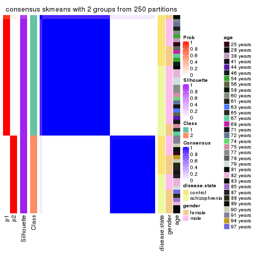
consensus_heatmap(res, k = 3)
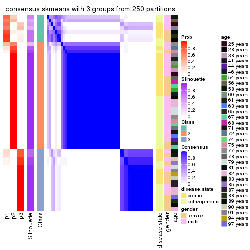
consensus_heatmap(res, k = 4)
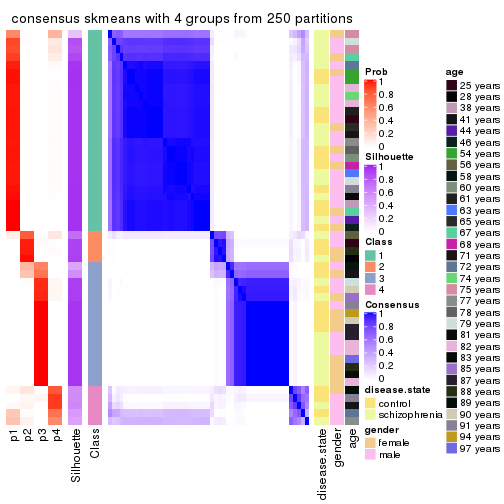
consensus_heatmap(res, k = 5)
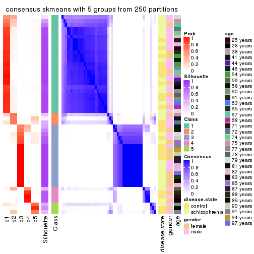
consensus_heatmap(res, k = 6)
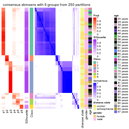
Heatmaps for the membership of samples in all partitions to see how consistent they are:
membership_heatmap(res, k = 2)
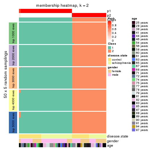
membership_heatmap(res, k = 3)
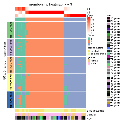
membership_heatmap(res, k = 4)
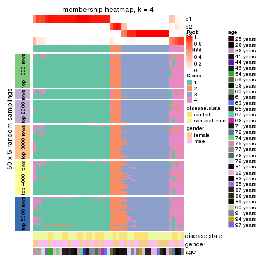
membership_heatmap(res, k = 5)
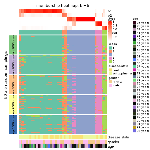
membership_heatmap(res, k = 6)
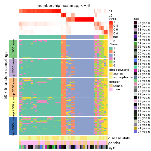
As soon as we have had the classes for columns, we can look for signatures which are significantly different between classes which can be candidate marks for certain classes. Following are the heatmaps for signatures.
Signature heatmaps where rows are scaled:
get_signatures(res, k = 2)
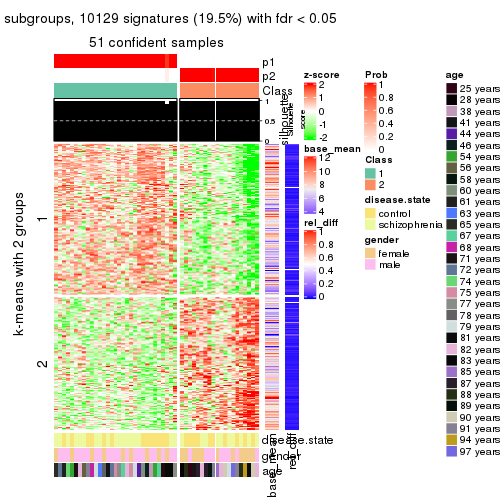
get_signatures(res, k = 3)
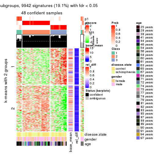
get_signatures(res, k = 4)
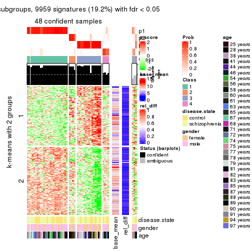
get_signatures(res, k = 5)
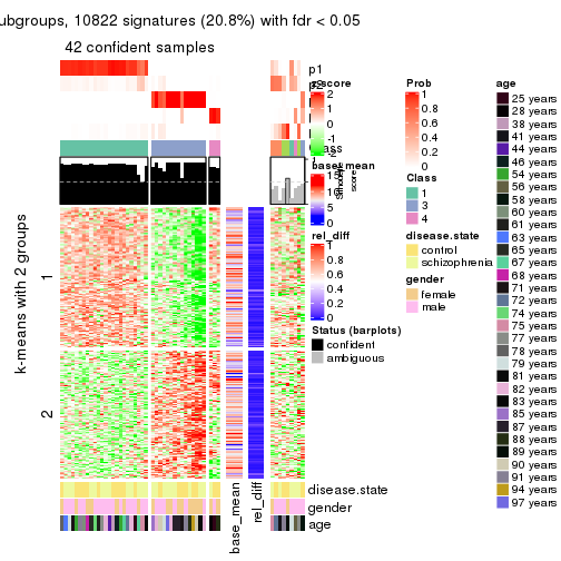
get_signatures(res, k = 6)
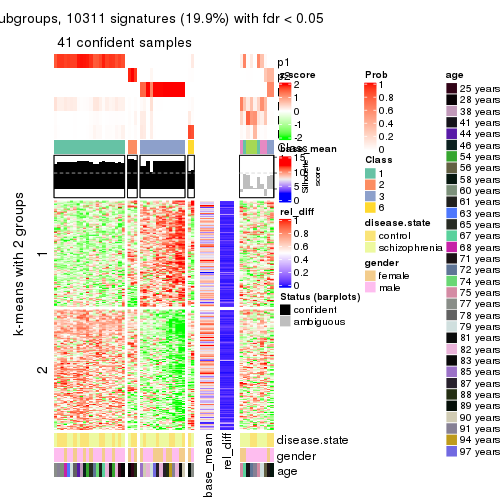
Signature heatmaps where rows are not scaled:
get_signatures(res, k = 2, scale_rows = FALSE)
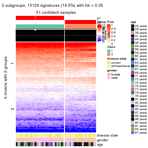
get_signatures(res, k = 3, scale_rows = FALSE)
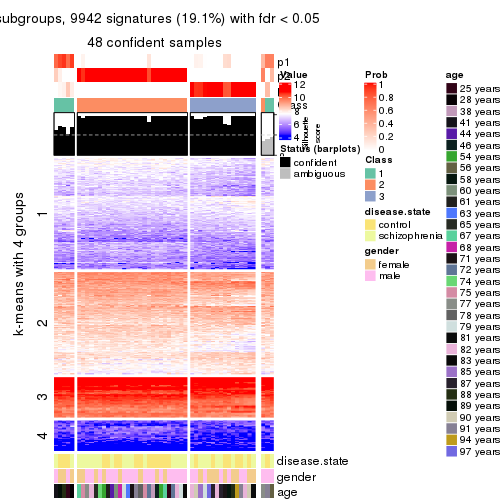
get_signatures(res, k = 4, scale_rows = FALSE)
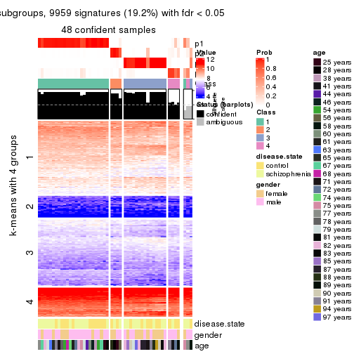
get_signatures(res, k = 5, scale_rows = FALSE)
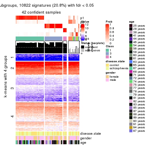
get_signatures(res, k = 6, scale_rows = FALSE)
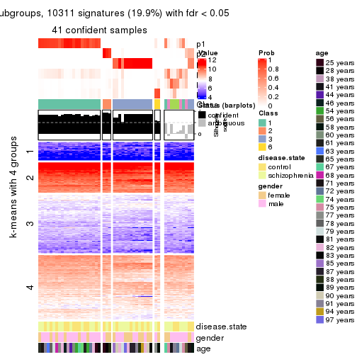
Compare the overlap of signatures from different k:
compare_signatures(res)
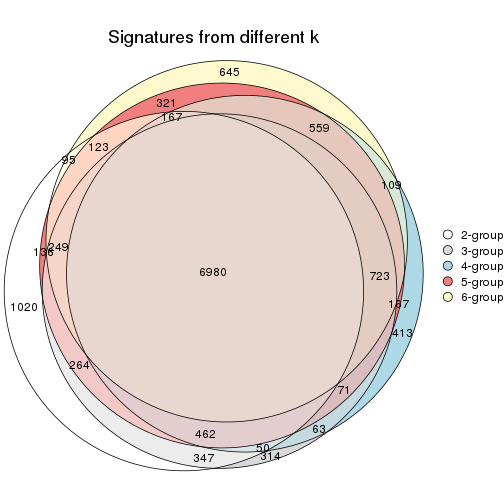
get_signature() returns a data frame invisibly. TO get the list of signatures, the function
call should be assigned to a variable explicitly. In following code, if plot argument is set
to FALSE, no heatmap is plotted while only the differential analysis is performed.
# code only for demonstration
tb = get_signature(res, k = ..., plot = FALSE)
An example of the output of tb is:
#> which_row fdr mean_1 mean_2 scaled_mean_1 scaled_mean_2 km
#> 1 38 0.042760348 8.373488 9.131774 -0.5533452 0.5164555 1
#> 2 40 0.018707592 7.106213 8.469186 -0.6173731 0.5762149 1
#> 3 55 0.019134737 10.221463 11.207825 -0.6159697 0.5749050 1
#> 4 59 0.006059896 5.921854 7.869574 -0.6899429 0.6439467 1
#> 5 60 0.018055526 8.928898 10.211722 -0.6204761 0.5791110 1
#> 6 98 0.009384629 15.714769 14.887706 0.6635654 -0.6193277 2
...
The columns in tb are:
which_row: row indices corresponding to the input matrix.fdr: FDR for the differential test. mean_x: The mean value in group x.scaled_mean_x: The mean value in group x after rows are scaled.km: Row groups if k-means clustering is applied to rows.UMAP plot which shows how samples are separated.
dimension_reduction(res, k = 2, method = "UMAP")
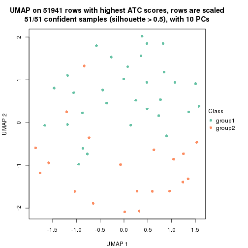
dimension_reduction(res, k = 3, method = "UMAP")
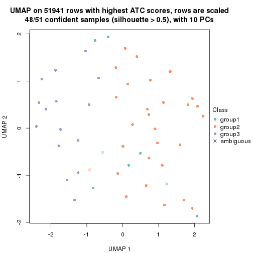
dimension_reduction(res, k = 4, method = "UMAP")
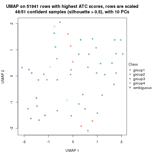
dimension_reduction(res, k = 5, method = "UMAP")
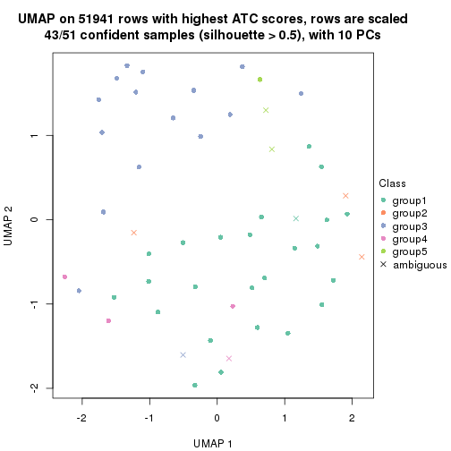
dimension_reduction(res, k = 6, method = "UMAP")
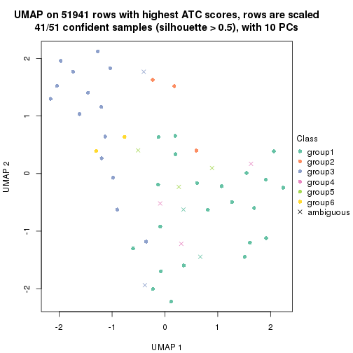
Following heatmap shows how subgroups are split when increasing k:
collect_classes(res)
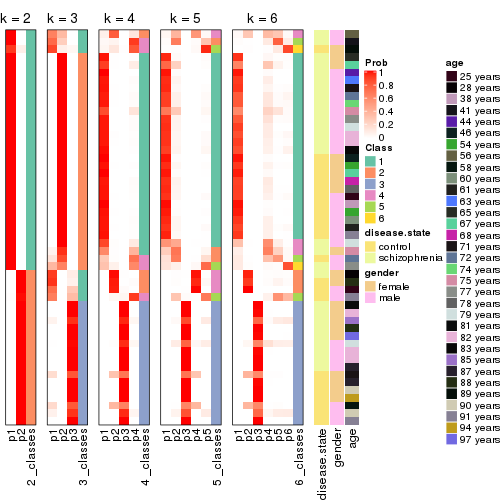
Test correlation between subgroups and known annotations. If the known annotation is numeric, one-way ANOVA test is applied, and if the known annotation is discrete, chi-squared contingency table test is applied.
test_to_known_factors(res)
#> n disease.state(p) gender(p) age(p) k
#> ATC:skmeans 51 0.782 0.119 0.280 2
#> ATC:skmeans 48 0.797 0.157 0.219 3
#> ATC:skmeans 48 0.651 0.207 0.317 4
#> ATC:skmeans 43 0.593 0.133 0.165 5
#> ATC:skmeans 41 0.738 0.252 0.443 6
If matrix rows can be associated to genes, consider to use functional_enrichment(res,
...) to perform function enrichment for the signature genes. See this vignette for more detailed explanations.
The object with results only for a single top-value method and a single partition method can be extracted as:
res = res_list["ATC", "pam"]
# you can also extract it by
# res = res_list["ATC:pam"]
A summary of res and all the functions that can be applied to it:
res
#> A 'ConsensusPartition' object with k = 2, 3, 4, 5, 6.
#> On a matrix with 51941 rows and 51 columns.
#> Top rows (1000, 2000, 3000, 4000, 5000) are extracted by 'ATC' method.
#> Subgroups are detected by 'pam' method.
#> Performed in total 1250 partitions by row resampling.
#> Best k for subgroups seems to be 2.
#>
#> Following methods can be applied to this 'ConsensusPartition' object:
#> [1] "cola_report" "collect_classes" "collect_plots"
#> [4] "collect_stats" "colnames" "compare_signatures"
#> [7] "consensus_heatmap" "dimension_reduction" "functional_enrichment"
#> [10] "get_anno_col" "get_anno" "get_classes"
#> [13] "get_consensus" "get_matrix" "get_membership"
#> [16] "get_param" "get_signatures" "get_stats"
#> [19] "is_best_k" "is_stable_k" "membership_heatmap"
#> [22] "ncol" "nrow" "plot_ecdf"
#> [25] "rownames" "select_partition_number" "show"
#> [28] "suggest_best_k" "test_to_known_factors"
collect_plots() function collects all the plots made from res for all k (number of partitions)
into one single page to provide an easy and fast comparison between different k.
collect_plots(res)
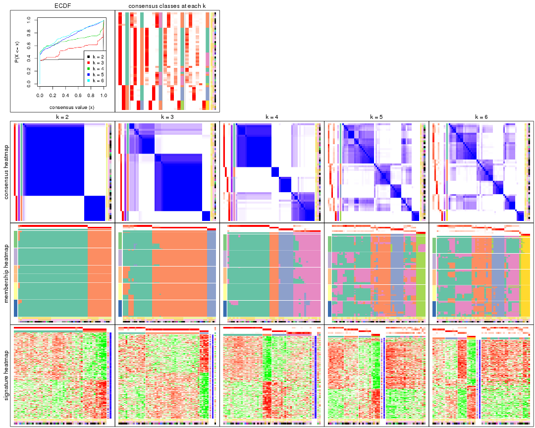
The plots are:
k and the heatmap of
predicted classes for each k.k.k.k.All the plots in panels can be made by individual functions and they are plotted later in this section.
select_partition_number() produces several plots showing different
statistics for choosing “optimized” k. There are following statistics:
k;k, the area increased is defined as \(A_k - A_{k-1}\).The detailed explanations of these statistics can be found in the cola vignette.
Generally speaking, lower PAC score, higher mean silhouette score or higher
concordance corresponds to better partition. Rand index and Jaccard index
measure how similar the current partition is compared to partition with k-1.
If they are too similar, we won't accept k is better than k-1.
select_partition_number(res)
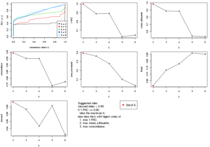
The numeric values for all these statistics can be obtained by get_stats().
get_stats(res)
#> k 1-PAC mean_silhouette concordance area_increased Rand Jaccard
#> 2 2 1.000 0.985 0.993 0.3943 0.613 0.613
#> 3 3 0.889 0.887 0.952 0.3604 0.730 0.593
#> 4 4 0.892 0.884 0.950 0.2765 0.780 0.548
#> 5 5 0.628 0.536 0.743 0.1020 0.861 0.602
#> 6 6 0.644 0.528 0.772 0.0308 0.853 0.524
suggest_best_k() suggests the best \(k\) based on these statistics. The rules are as follows:
suggest_best_k(res)
#> [1] 2
Following shows the table of the partitions (You need to click the show/hide
code output link to see it). The membership matrix (columns with name p*)
is inferred by
clue::cl_consensus()
function with the SE method. Basically the value in the membership matrix
represents the probability to belong to a certain group. The finall class
label for an item is determined with the group with highest probability it
belongs to.
In get_classes() function, the entropy is calculated from the membership
matrix and the silhouette score is calculated from the consensus matrix.
cbind(get_classes(res, k = 2), get_membership(res, k = 2))
#> class entropy silhouette p1 p2
#> GSM439800 1 0.000 0.991 1.000 0.000
#> GSM439790 1 0.000 0.991 1.000 0.000
#> GSM439827 1 0.000 0.991 1.000 0.000
#> GSM439811 1 0.000 0.991 1.000 0.000
#> GSM439795 2 0.000 1.000 0.000 1.000
#> GSM439805 2 0.000 1.000 0.000 1.000
#> GSM439781 1 0.311 0.935 0.944 0.056
#> GSM439807 2 0.000 1.000 0.000 1.000
#> GSM439820 2 0.000 1.000 0.000 1.000
#> GSM439784 1 0.000 0.991 1.000 0.000
#> GSM439824 1 0.000 0.991 1.000 0.000
#> GSM439794 1 0.000 0.991 1.000 0.000
#> GSM439809 1 0.000 0.991 1.000 0.000
#> GSM439785 1 0.000 0.991 1.000 0.000
#> GSM439803 1 0.000 0.991 1.000 0.000
#> GSM439778 1 0.000 0.991 1.000 0.000
#> GSM439791 1 0.000 0.991 1.000 0.000
#> GSM439786 1 0.000 0.991 1.000 0.000
#> GSM439828 1 0.000 0.991 1.000 0.000
#> GSM439806 1 0.000 0.991 1.000 0.000
#> GSM439815 1 0.000 0.991 1.000 0.000
#> GSM439817 1 0.000 0.991 1.000 0.000
#> GSM439796 1 0.000 0.991 1.000 0.000
#> GSM439798 2 0.000 1.000 0.000 1.000
#> GSM439821 2 0.000 1.000 0.000 1.000
#> GSM439823 1 0.000 0.991 1.000 0.000
#> GSM439813 1 0.000 0.991 1.000 0.000
#> GSM439801 2 0.000 1.000 0.000 1.000
#> GSM439810 1 0.000 0.991 1.000 0.000
#> GSM439783 1 0.000 0.991 1.000 0.000
#> GSM439826 1 0.000 0.991 1.000 0.000
#> GSM439812 1 0.000 0.991 1.000 0.000
#> GSM439818 2 0.000 1.000 0.000 1.000
#> GSM439792 1 0.000 0.991 1.000 0.000
#> GSM439802 2 0.000 1.000 0.000 1.000
#> GSM439825 1 0.000 0.991 1.000 0.000
#> GSM439780 1 0.000 0.991 1.000 0.000
#> GSM439787 2 0.000 1.000 0.000 1.000
#> GSM439808 2 0.000 1.000 0.000 1.000
#> GSM439804 1 0.000 0.991 1.000 0.000
#> GSM439822 1 0.000 0.991 1.000 0.000
#> GSM439816 1 0.000 0.991 1.000 0.000
#> GSM439789 1 0.000 0.991 1.000 0.000
#> GSM439799 2 0.000 1.000 0.000 1.000
#> GSM439814 1 0.000 0.991 1.000 0.000
#> GSM439782 1 0.000 0.991 1.000 0.000
#> GSM439779 1 0.000 0.991 1.000 0.000
#> GSM439793 1 0.861 0.608 0.716 0.284
#> GSM439788 1 0.000 0.991 1.000 0.000
#> GSM439797 1 0.000 0.991 1.000 0.000
#> GSM439819 2 0.000 1.000 0.000 1.000
cbind(get_classes(res, k = 3), get_membership(res, k = 3))
#> class entropy silhouette p1 p2 p3
#> GSM439800 1 0.5591 0.596 0.696 0.304 0.000
#> GSM439790 2 0.0000 0.984 0.000 1.000 0.000
#> GSM439827 2 0.0000 0.984 0.000 1.000 0.000
#> GSM439811 2 0.2878 0.888 0.096 0.904 0.000
#> GSM439795 3 0.0000 1.000 0.000 0.000 1.000
#> GSM439805 1 0.0000 0.788 1.000 0.000 0.000
#> GSM439781 1 0.0000 0.788 1.000 0.000 0.000
#> GSM439807 1 0.2878 0.708 0.904 0.000 0.096
#> GSM439820 1 0.0000 0.788 1.000 0.000 0.000
#> GSM439784 2 0.2878 0.888 0.096 0.904 0.000
#> GSM439824 2 0.0000 0.984 0.000 1.000 0.000
#> GSM439794 2 0.2878 0.888 0.096 0.904 0.000
#> GSM439809 2 0.0000 0.984 0.000 1.000 0.000
#> GSM439785 2 0.0000 0.984 0.000 1.000 0.000
#> GSM439803 2 0.0000 0.984 0.000 1.000 0.000
#> GSM439778 2 0.0000 0.984 0.000 1.000 0.000
#> GSM439791 2 0.0000 0.984 0.000 1.000 0.000
#> GSM439786 2 0.1411 0.953 0.036 0.964 0.000
#> GSM439828 2 0.0000 0.984 0.000 1.000 0.000
#> GSM439806 2 0.0000 0.984 0.000 1.000 0.000
#> GSM439815 2 0.0237 0.981 0.004 0.996 0.000
#> GSM439817 1 0.5098 0.623 0.752 0.248 0.000
#> GSM439796 2 0.0000 0.984 0.000 1.000 0.000
#> GSM439798 1 0.0000 0.788 1.000 0.000 0.000
#> GSM439821 3 0.0000 1.000 0.000 0.000 1.000
#> GSM439823 2 0.0000 0.984 0.000 1.000 0.000
#> GSM439813 2 0.0000 0.984 0.000 1.000 0.000
#> GSM439801 1 0.1643 0.758 0.956 0.000 0.044
#> GSM439810 2 0.0000 0.984 0.000 1.000 0.000
#> GSM439783 2 0.0000 0.984 0.000 1.000 0.000
#> GSM439826 2 0.0000 0.984 0.000 1.000 0.000
#> GSM439812 2 0.0000 0.984 0.000 1.000 0.000
#> GSM439818 1 0.0000 0.788 1.000 0.000 0.000
#> GSM439792 2 0.0000 0.984 0.000 1.000 0.000
#> GSM439802 1 0.0000 0.788 1.000 0.000 0.000
#> GSM439825 1 0.5621 0.591 0.692 0.308 0.000
#> GSM439780 1 0.6225 0.361 0.568 0.432 0.000
#> GSM439787 3 0.0000 1.000 0.000 0.000 1.000
#> GSM439808 3 0.0000 1.000 0.000 0.000 1.000
#> GSM439804 2 0.0000 0.984 0.000 1.000 0.000
#> GSM439822 1 0.5591 0.596 0.696 0.304 0.000
#> GSM439816 2 0.0000 0.984 0.000 1.000 0.000
#> GSM439789 2 0.0000 0.984 0.000 1.000 0.000
#> GSM439799 1 0.0000 0.788 1.000 0.000 0.000
#> GSM439814 2 0.0000 0.984 0.000 1.000 0.000
#> GSM439782 2 0.0000 0.984 0.000 1.000 0.000
#> GSM439779 2 0.2261 0.920 0.068 0.932 0.000
#> GSM439793 1 0.0000 0.788 1.000 0.000 0.000
#> GSM439788 1 0.5497 0.579 0.708 0.292 0.000
#> GSM439797 2 0.0000 0.984 0.000 1.000 0.000
#> GSM439819 3 0.0000 1.000 0.000 0.000 1.000
cbind(get_classes(res, k = 4), get_membership(res, k = 4))
#> class entropy silhouette p1 p2 p3 p4
#> GSM439800 4 0.4456 0.539 0.004 0 0.280 0.716
#> GSM439790 1 0.1474 0.931 0.948 0 0.000 0.052
#> GSM439827 1 0.0000 0.964 1.000 0 0.000 0.000
#> GSM439811 1 0.4916 0.191 0.576 0 0.000 0.424
#> GSM439795 2 0.0000 1.000 0.000 1 0.000 0.000
#> GSM439805 3 0.0000 0.983 0.000 0 1.000 0.000
#> GSM439781 4 0.1867 0.800 0.000 0 0.072 0.928
#> GSM439807 3 0.0000 0.983 0.000 0 1.000 0.000
#> GSM439820 3 0.0000 0.983 0.000 0 1.000 0.000
#> GSM439784 4 0.0000 0.835 0.000 0 0.000 1.000
#> GSM439824 1 0.0000 0.964 1.000 0 0.000 0.000
#> GSM439794 4 0.1118 0.828 0.036 0 0.000 0.964
#> GSM439809 1 0.0000 0.964 1.000 0 0.000 0.000
#> GSM439785 1 0.0000 0.964 1.000 0 0.000 0.000
#> GSM439803 4 0.3942 0.691 0.236 0 0.000 0.764
#> GSM439778 4 0.4955 0.285 0.444 0 0.000 0.556
#> GSM439791 1 0.1022 0.939 0.968 0 0.000 0.032
#> GSM439786 4 0.4193 0.657 0.268 0 0.000 0.732
#> GSM439828 1 0.0000 0.964 1.000 0 0.000 0.000
#> GSM439806 1 0.0000 0.964 1.000 0 0.000 0.000
#> GSM439815 4 0.3907 0.695 0.232 0 0.000 0.768
#> GSM439817 4 0.0188 0.834 0.000 0 0.004 0.996
#> GSM439796 1 0.1557 0.927 0.944 0 0.000 0.056
#> GSM439798 3 0.0000 0.983 0.000 0 1.000 0.000
#> GSM439821 2 0.0000 1.000 0.000 1 0.000 0.000
#> GSM439823 1 0.0000 0.964 1.000 0 0.000 0.000
#> GSM439813 1 0.0000 0.964 1.000 0 0.000 0.000
#> GSM439801 3 0.0000 0.983 0.000 0 1.000 0.000
#> GSM439810 1 0.0000 0.964 1.000 0 0.000 0.000
#> GSM439783 1 0.0000 0.964 1.000 0 0.000 0.000
#> GSM439826 1 0.0000 0.964 1.000 0 0.000 0.000
#> GSM439812 1 0.0000 0.964 1.000 0 0.000 0.000
#> GSM439818 3 0.2345 0.876 0.000 0 0.900 0.100
#> GSM439792 1 0.0000 0.964 1.000 0 0.000 0.000
#> GSM439802 3 0.0000 0.983 0.000 0 1.000 0.000
#> GSM439825 4 0.0000 0.835 0.000 0 0.000 1.000
#> GSM439780 4 0.0000 0.835 0.000 0 0.000 1.000
#> GSM439787 2 0.0000 1.000 0.000 1 0.000 0.000
#> GSM439808 2 0.0000 1.000 0.000 1 0.000 0.000
#> GSM439804 1 0.1557 0.927 0.944 0 0.000 0.056
#> GSM439822 4 0.0000 0.835 0.000 0 0.000 1.000
#> GSM439816 1 0.0000 0.964 1.000 0 0.000 0.000
#> GSM439789 1 0.0000 0.964 1.000 0 0.000 0.000
#> GSM439799 3 0.0000 0.983 0.000 0 1.000 0.000
#> GSM439814 1 0.0000 0.964 1.000 0 0.000 0.000
#> GSM439782 1 0.1557 0.927 0.944 0 0.000 0.056
#> GSM439779 4 0.2216 0.801 0.092 0 0.000 0.908
#> GSM439793 4 0.1557 0.807 0.000 0 0.056 0.944
#> GSM439788 4 0.0000 0.835 0.000 0 0.000 1.000
#> GSM439797 1 0.0921 0.948 0.972 0 0.000 0.028
#> GSM439819 2 0.0000 1.000 0.000 1 0.000 0.000
cbind(get_classes(res, k = 5), get_membership(res, k = 5))
#> class entropy silhouette p1 p2 p3 p4 p5
#> GSM439800 2 0.5462 0.5158 0.000 0.652 0.136 0.212 0.000
#> GSM439790 1 0.3671 0.5089 0.756 0.008 0.000 0.236 0.000
#> GSM439827 1 0.4066 0.5219 0.768 0.044 0.000 0.188 0.000
#> GSM439811 2 0.3774 0.4053 0.296 0.704 0.000 0.000 0.000
#> GSM439795 5 0.0000 0.9794 0.000 0.000 0.000 0.000 1.000
#> GSM439805 3 0.0000 0.9393 0.000 0.000 1.000 0.000 0.000
#> GSM439781 2 0.1043 0.7715 0.000 0.960 0.040 0.000 0.000
#> GSM439807 3 0.2959 0.8743 0.000 0.036 0.864 0.100 0.000
#> GSM439820 3 0.2891 0.7966 0.000 0.176 0.824 0.000 0.000
#> GSM439784 2 0.5005 0.4155 0.064 0.660 0.000 0.276 0.000
#> GSM439824 1 0.2929 0.4821 0.820 0.000 0.000 0.180 0.000
#> GSM439794 4 0.4547 0.3419 0.012 0.400 0.000 0.588 0.000
#> GSM439809 1 0.4042 0.5117 0.756 0.032 0.000 0.212 0.000
#> GSM439785 1 0.4305 0.0377 0.512 0.000 0.000 0.488 0.000
#> GSM439803 4 0.5701 0.5262 0.124 0.272 0.000 0.604 0.000
#> GSM439778 4 0.6210 0.3806 0.276 0.184 0.000 0.540 0.000
#> GSM439791 1 0.4219 0.4766 0.716 0.024 0.000 0.260 0.000
#> GSM439786 4 0.6858 0.2671 0.244 0.300 0.008 0.448 0.000
#> GSM439828 1 0.3452 0.5162 0.756 0.000 0.000 0.244 0.000
#> GSM439806 1 0.0404 0.5331 0.988 0.000 0.000 0.012 0.000
#> GSM439815 1 0.6814 -0.3450 0.352 0.304 0.000 0.344 0.000
#> GSM439817 2 0.0794 0.7735 0.000 0.972 0.028 0.000 0.000
#> GSM439796 4 0.4546 -0.0506 0.460 0.008 0.000 0.532 0.000
#> GSM439798 3 0.0963 0.9286 0.000 0.036 0.964 0.000 0.000
#> GSM439821 5 0.0000 0.9794 0.000 0.000 0.000 0.000 1.000
#> GSM439823 1 0.4219 0.2273 0.584 0.000 0.000 0.416 0.000
#> GSM439813 1 0.2329 0.5477 0.876 0.000 0.000 0.124 0.000
#> GSM439801 3 0.0000 0.9393 0.000 0.000 1.000 0.000 0.000
#> GSM439810 1 0.2929 0.4821 0.820 0.000 0.000 0.180 0.000
#> GSM439783 1 0.4294 0.0665 0.532 0.000 0.000 0.468 0.000
#> GSM439826 1 0.3949 0.3657 0.668 0.000 0.000 0.332 0.000
#> GSM439812 1 0.2966 0.5425 0.816 0.000 0.000 0.184 0.000
#> GSM439818 2 0.4561 -0.1151 0.000 0.504 0.488 0.008 0.000
#> GSM439792 1 0.3452 0.5162 0.756 0.000 0.000 0.244 0.000
#> GSM439802 3 0.0000 0.9393 0.000 0.000 1.000 0.000 0.000
#> GSM439825 2 0.1121 0.7670 0.000 0.956 0.000 0.044 0.000
#> GSM439780 2 0.2104 0.7664 0.000 0.916 0.024 0.060 0.000
#> GSM439787 5 0.0000 0.9794 0.000 0.000 0.000 0.000 1.000
#> GSM439808 5 0.0510 0.9755 0.000 0.000 0.000 0.016 0.984
#> GSM439804 1 0.4562 0.1613 0.496 0.008 0.000 0.496 0.000
#> GSM439822 2 0.1608 0.7578 0.000 0.928 0.000 0.072 0.000
#> GSM439816 1 0.2929 0.4821 0.820 0.000 0.000 0.180 0.000
#> GSM439789 1 0.4227 0.2677 0.580 0.000 0.000 0.420 0.000
#> GSM439799 3 0.0794 0.9222 0.000 0.028 0.972 0.000 0.000
#> GSM439814 1 0.2929 0.4821 0.820 0.000 0.000 0.180 0.000
#> GSM439782 4 0.4562 -0.0968 0.492 0.008 0.000 0.500 0.000
#> GSM439779 4 0.4557 0.3343 0.012 0.404 0.000 0.584 0.000
#> GSM439793 2 0.0963 0.7725 0.000 0.964 0.036 0.000 0.000
#> GSM439788 2 0.3099 0.7304 0.000 0.848 0.028 0.124 0.000
#> GSM439797 1 0.3508 0.5108 0.748 0.000 0.000 0.252 0.000
#> GSM439819 5 0.2020 0.9293 0.000 0.000 0.000 0.100 0.900
cbind(get_classes(res, k = 6), get_membership(res, k = 6))
#> class entropy silhouette p1 p2 p3 p4 p5 p6
#> GSM439800 2 0.6772 0.4280 0.188 0.580 0.104 0.080 0.048 0.000
#> GSM439790 1 0.3812 0.4649 0.712 0.016 0.000 0.268 0.004 0.000
#> GSM439827 1 0.4495 0.3677 0.660 0.064 0.000 0.276 0.000 0.000
#> GSM439811 2 0.3806 0.4819 0.200 0.752 0.000 0.048 0.000 0.000
#> GSM439795 6 0.0000 0.9591 0.000 0.000 0.000 0.000 0.000 1.000
#> GSM439805 3 0.0000 0.9088 0.000 0.000 1.000 0.000 0.000 0.000
#> GSM439781 2 0.1991 0.7235 0.000 0.920 0.044 0.024 0.012 0.000
#> GSM439807 3 0.3390 0.7918 0.000 0.008 0.808 0.032 0.152 0.000
#> GSM439820 3 0.3516 0.7143 0.000 0.172 0.792 0.024 0.012 0.000
#> GSM439784 2 0.5721 0.3115 0.188 0.556 0.000 0.248 0.008 0.000
#> GSM439824 4 0.2996 0.6577 0.228 0.000 0.000 0.772 0.000 0.000
#> GSM439794 1 0.5866 0.0438 0.516 0.292 0.000 0.184 0.008 0.000
#> GSM439809 1 0.3606 0.4615 0.728 0.016 0.000 0.256 0.000 0.000
#> GSM439785 1 0.0458 0.4748 0.984 0.000 0.000 0.016 0.000 0.000
#> GSM439803 1 0.5519 0.1479 0.580 0.264 0.000 0.148 0.008 0.000
#> GSM439778 1 0.3580 0.3373 0.772 0.196 0.000 0.028 0.004 0.000
#> GSM439791 1 0.3905 0.4407 0.668 0.016 0.000 0.316 0.000 0.000
#> GSM439786 5 0.3729 0.0000 0.024 0.040 0.000 0.136 0.800 0.000
#> GSM439828 1 0.3175 0.4655 0.744 0.000 0.000 0.256 0.000 0.000
#> GSM439806 4 0.3862 0.1628 0.476 0.000 0.000 0.524 0.000 0.000
#> GSM439815 4 0.6281 -0.2373 0.284 0.308 0.000 0.400 0.008 0.000
#> GSM439817 2 0.1777 0.7269 0.000 0.932 0.032 0.024 0.012 0.000
#> GSM439796 1 0.1010 0.4697 0.960 0.036 0.000 0.000 0.004 0.000
#> GSM439798 3 0.1251 0.8918 0.000 0.008 0.956 0.024 0.012 0.000
#> GSM439821 6 0.0000 0.9591 0.000 0.000 0.000 0.000 0.000 1.000
#> GSM439823 1 0.1765 0.4773 0.904 0.000 0.000 0.096 0.000 0.000
#> GSM439813 1 0.3975 0.1667 0.600 0.008 0.000 0.392 0.000 0.000
#> GSM439801 3 0.0000 0.9088 0.000 0.000 1.000 0.000 0.000 0.000
#> GSM439810 4 0.2996 0.6577 0.228 0.000 0.000 0.772 0.000 0.000
#> GSM439783 1 0.0713 0.4682 0.972 0.000 0.000 0.028 0.000 0.000
#> GSM439826 4 0.3747 0.5227 0.396 0.000 0.000 0.604 0.000 0.000
#> GSM439812 1 0.3409 0.4155 0.700 0.000 0.000 0.300 0.000 0.000
#> GSM439818 2 0.4665 0.3735 0.000 0.632 0.316 0.012 0.040 0.000
#> GSM439792 1 0.3175 0.4655 0.744 0.000 0.000 0.256 0.000 0.000
#> GSM439802 3 0.0000 0.9088 0.000 0.000 1.000 0.000 0.000 0.000
#> GSM439825 2 0.1692 0.7160 0.008 0.932 0.000 0.012 0.048 0.000
#> GSM439780 2 0.2487 0.7032 0.008 0.892 0.028 0.068 0.004 0.000
#> GSM439787 6 0.0000 0.9591 0.000 0.000 0.000 0.000 0.000 1.000
#> GSM439808 6 0.0603 0.9524 0.000 0.000 0.000 0.004 0.016 0.980
#> GSM439804 1 0.4407 -0.4196 0.492 0.024 0.000 0.484 0.000 0.000
#> GSM439822 2 0.1692 0.7160 0.008 0.932 0.000 0.012 0.048 0.000
#> GSM439816 4 0.2996 0.6577 0.228 0.000 0.000 0.772 0.000 0.000
#> GSM439789 4 0.3847 0.4310 0.456 0.000 0.000 0.544 0.000 0.000
#> GSM439799 3 0.0790 0.8851 0.000 0.032 0.968 0.000 0.000 0.000
#> GSM439814 4 0.2996 0.6577 0.228 0.000 0.000 0.772 0.000 0.000
#> GSM439782 1 0.1552 0.4610 0.940 0.036 0.000 0.020 0.004 0.000
#> GSM439779 1 0.5923 0.0151 0.496 0.312 0.000 0.184 0.008 0.000
#> GSM439793 2 0.1777 0.7269 0.000 0.932 0.032 0.024 0.012 0.000
#> GSM439788 2 0.3843 0.6059 0.008 0.772 0.028 0.184 0.008 0.000
#> GSM439797 1 0.3265 0.4712 0.748 0.000 0.000 0.248 0.004 0.000
#> GSM439819 6 0.2513 0.8507 0.000 0.000 0.000 0.008 0.140 0.852
Heatmaps for the consensus matrix. It visualizes the probability of two samples to be in a same group.
consensus_heatmap(res, k = 2)
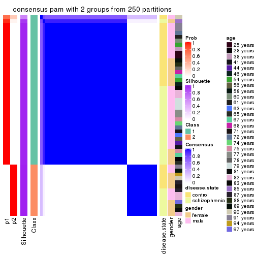
consensus_heatmap(res, k = 3)
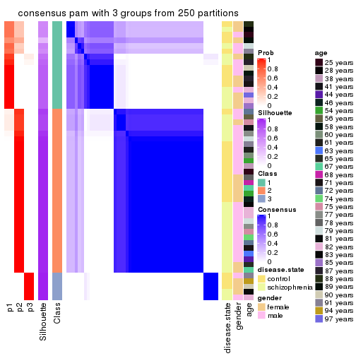
consensus_heatmap(res, k = 4)
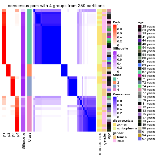
consensus_heatmap(res, k = 5)
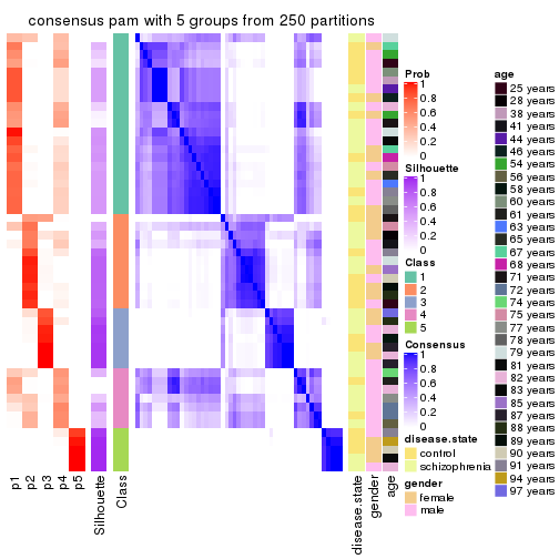
consensus_heatmap(res, k = 6)
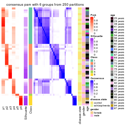
Heatmaps for the membership of samples in all partitions to see how consistent they are:
membership_heatmap(res, k = 2)
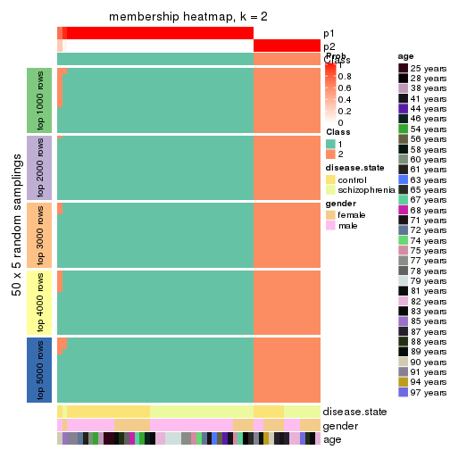
membership_heatmap(res, k = 3)
membership_heatmap(res, k = 4)
membership_heatmap(res, k = 5)
membership_heatmap(res, k = 6)
As soon as we have had the classes for columns, we can look for signatures which are significantly different between classes which can be candidate marks for certain classes. Following are the heatmaps for signatures.
Signature heatmaps where rows are scaled:
get_signatures(res, k = 2)

get_signatures(res, k = 3)
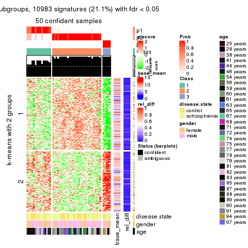
get_signatures(res, k = 4)
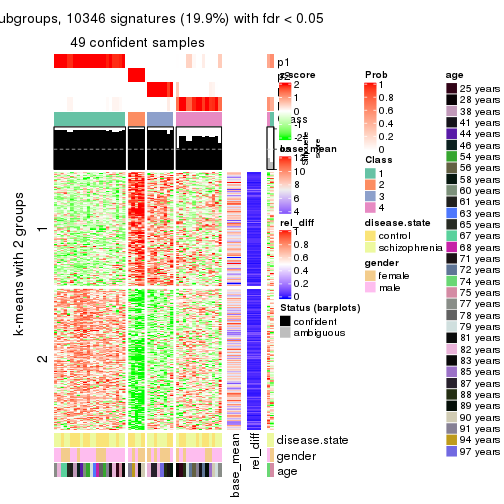
get_signatures(res, k = 5)
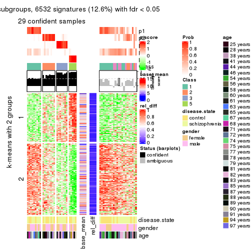
get_signatures(res, k = 6)
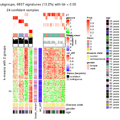
Signature heatmaps where rows are not scaled:
get_signatures(res, k = 2, scale_rows = FALSE)
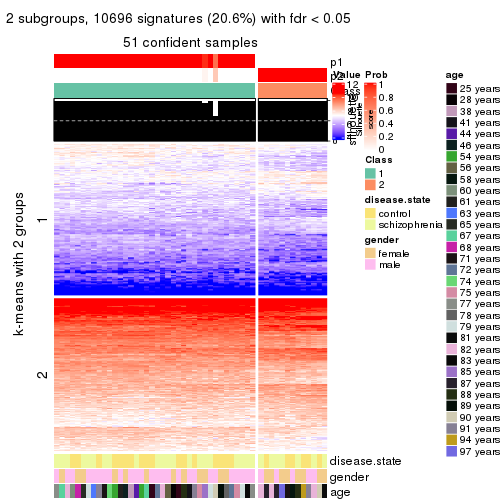
get_signatures(res, k = 3, scale_rows = FALSE)
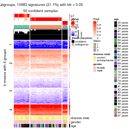
get_signatures(res, k = 4, scale_rows = FALSE)
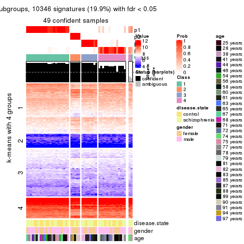
get_signatures(res, k = 5, scale_rows = FALSE)
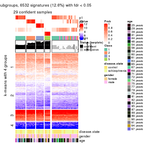
get_signatures(res, k = 6, scale_rows = FALSE)
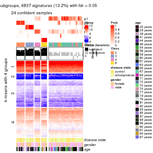
Compare the overlap of signatures from different k:
compare_signatures(res)
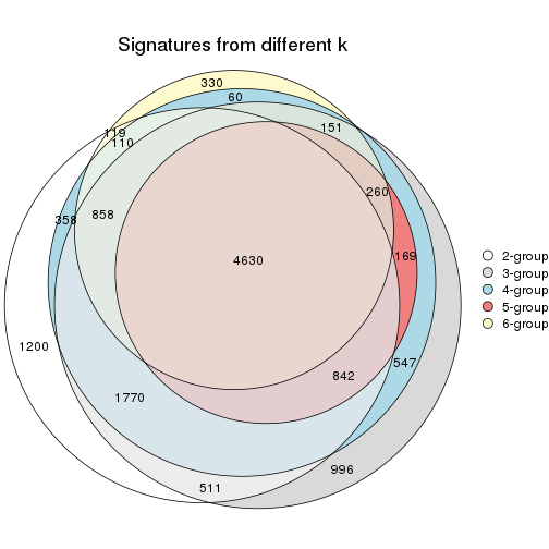
get_signature() returns a data frame invisibly. TO get the list of signatures, the function
call should be assigned to a variable explicitly. In following code, if plot argument is set
to FALSE, no heatmap is plotted while only the differential analysis is performed.
# code only for demonstration
tb = get_signature(res, k = ..., plot = FALSE)
An example of the output of tb is:
#> which_row fdr mean_1 mean_2 scaled_mean_1 scaled_mean_2 km
#> 1 38 0.042760348 8.373488 9.131774 -0.5533452 0.5164555 1
#> 2 40 0.018707592 7.106213 8.469186 -0.6173731 0.5762149 1
#> 3 55 0.019134737 10.221463 11.207825 -0.6159697 0.5749050 1
#> 4 59 0.006059896 5.921854 7.869574 -0.6899429 0.6439467 1
#> 5 60 0.018055526 8.928898 10.211722 -0.6204761 0.5791110 1
#> 6 98 0.009384629 15.714769 14.887706 0.6635654 -0.6193277 2
...
The columns in tb are:
which_row: row indices corresponding to the input matrix.fdr: FDR for the differential test. mean_x: The mean value in group x.scaled_mean_x: The mean value in group x after rows are scaled.km: Row groups if k-means clustering is applied to rows.UMAP plot which shows how samples are separated.
dimension_reduction(res, k = 2, method = "UMAP")

dimension_reduction(res, k = 3, method = "UMAP")
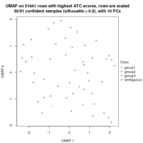
dimension_reduction(res, k = 4, method = "UMAP")
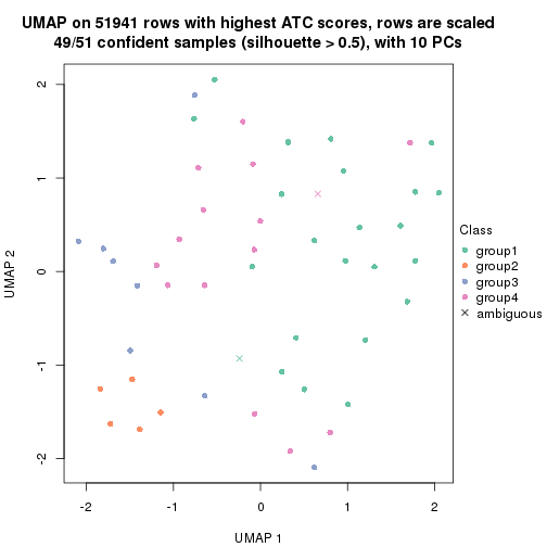
dimension_reduction(res, k = 5, method = "UMAP")
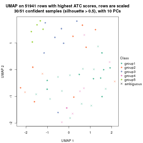
dimension_reduction(res, k = 6, method = "UMAP")
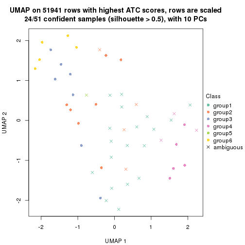
Following heatmap shows how subgroups are split when increasing k:
collect_classes(res)
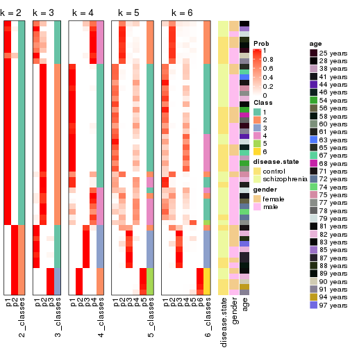
Test correlation between subgroups and known annotations. If the known annotation is numeric, one-way ANOVA test is applied, and if the known annotation is discrete, chi-squared contingency table test is applied.
test_to_known_factors(res)
#> n disease.state(p) gender(p) age(p) k
#> ATC:pam 51 1.000 0.114 0.405 2
#> ATC:pam 50 0.685 0.125 0.512 3
#> ATC:pam 49 0.848 0.272 0.463 4
#> ATC:pam 30 0.476 0.835 0.258 5
#> ATC:pam 24 0.260 0.877 0.331 6
If matrix rows can be associated to genes, consider to use functional_enrichment(res,
...) to perform function enrichment for the signature genes. See this vignette for more detailed explanations.
The object with results only for a single top-value method and a single partition method can be extracted as:
res = res_list["ATC", "mclust"]
# you can also extract it by
# res = res_list["ATC:mclust"]
A summary of res and all the functions that can be applied to it:
res
#> A 'ConsensusPartition' object with k = 2, 3, 4, 5, 6.
#> On a matrix with 51941 rows and 51 columns.
#> Top rows (1000, 2000, 3000, 4000, 5000) are extracted by 'ATC' method.
#> Subgroups are detected by 'mclust' method.
#> Performed in total 1250 partitions by row resampling.
#> Best k for subgroups seems to be 2.
#>
#> Following methods can be applied to this 'ConsensusPartition' object:
#> [1] "cola_report" "collect_classes" "collect_plots"
#> [4] "collect_stats" "colnames" "compare_signatures"
#> [7] "consensus_heatmap" "dimension_reduction" "functional_enrichment"
#> [10] "get_anno_col" "get_anno" "get_classes"
#> [13] "get_consensus" "get_matrix" "get_membership"
#> [16] "get_param" "get_signatures" "get_stats"
#> [19] "is_best_k" "is_stable_k" "membership_heatmap"
#> [22] "ncol" "nrow" "plot_ecdf"
#> [25] "rownames" "select_partition_number" "show"
#> [28] "suggest_best_k" "test_to_known_factors"
collect_plots() function collects all the plots made from res for all k (number of partitions)
into one single page to provide an easy and fast comparison between different k.
collect_plots(res)
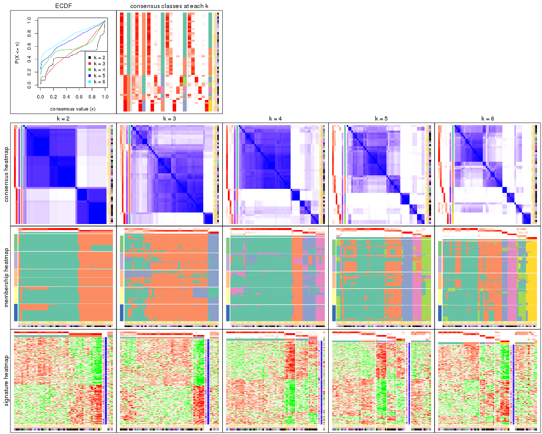
The plots are:
k and the heatmap of
predicted classes for each k.k.k.k.All the plots in panels can be made by individual functions and they are plotted later in this section.
select_partition_number() produces several plots showing different
statistics for choosing “optimized” k. There are following statistics:
k;k, the area increased is defined as \(A_k - A_{k-1}\).The detailed explanations of these statistics can be found in the cola vignette.
Generally speaking, lower PAC score, higher mean silhouette score or higher
concordance corresponds to better partition. Rand index and Jaccard index
measure how similar the current partition is compared to partition with k-1.
If they are too similar, we won't accept k is better than k-1.
select_partition_number(res)
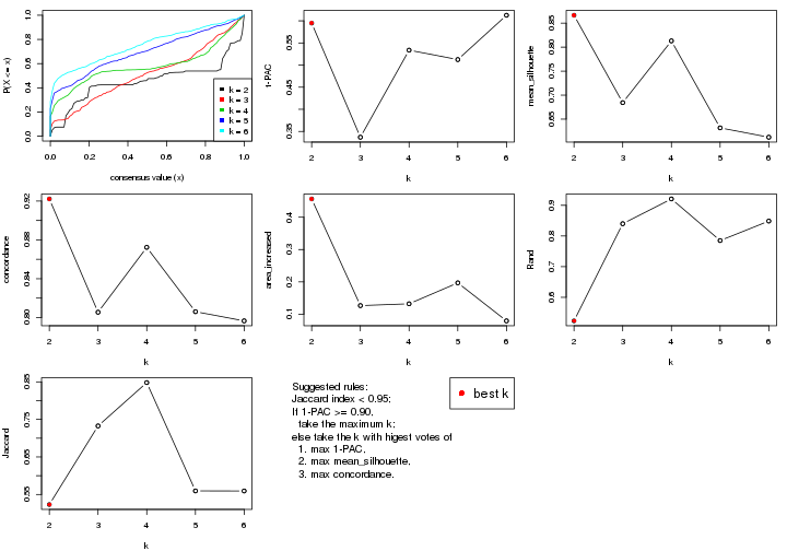
The numeric values for all these statistics can be obtained by get_stats().
get_stats(res)
#> k 1-PAC mean_silhouette concordance area_increased Rand Jaccard
#> 2 2 0.595 0.866 0.922 0.4566 0.523 0.523
#> 3 3 0.337 0.684 0.805 0.1266 0.840 0.733
#> 4 4 0.534 0.813 0.872 0.1322 0.921 0.848
#> 5 5 0.512 0.632 0.806 0.1969 0.785 0.559
#> 6 6 0.613 0.612 0.797 0.0793 0.849 0.559
suggest_best_k() suggests the best \(k\) based on these statistics. The rules are as follows:
suggest_best_k(res)
#> [1] 2
Following shows the table of the partitions (You need to click the show/hide
code output link to see it). The membership matrix (columns with name p*)
is inferred by
clue::cl_consensus()
function with the SE method. Basically the value in the membership matrix
represents the probability to belong to a certain group. The finall class
label for an item is determined with the group with highest probability it
belongs to.
In get_classes() function, the entropy is calculated from the membership
matrix and the silhouette score is calculated from the consensus matrix.
cbind(get_classes(res, k = 2), get_membership(res, k = 2))
#> class entropy silhouette p1 p2
#> GSM439800 2 0.3879 0.9397 0.076 0.924
#> GSM439790 1 0.0000 0.9066 1.000 0.000
#> GSM439827 1 0.5178 0.8951 0.884 0.116
#> GSM439811 1 0.5178 0.8951 0.884 0.116
#> GSM439795 2 0.0376 0.9114 0.004 0.996
#> GSM439805 2 0.3879 0.9397 0.076 0.924
#> GSM439781 2 0.5408 0.8889 0.124 0.876
#> GSM439807 2 0.0376 0.9114 0.004 0.996
#> GSM439820 2 0.3879 0.9397 0.076 0.924
#> GSM439784 1 0.0000 0.9066 1.000 0.000
#> GSM439824 1 0.5178 0.8951 0.884 0.116
#> GSM439794 2 0.9954 0.0959 0.460 0.540
#> GSM439809 1 0.0000 0.9066 1.000 0.000
#> GSM439785 1 0.0000 0.9066 1.000 0.000
#> GSM439803 1 0.4815 0.8990 0.896 0.104
#> GSM439778 1 0.5294 0.8918 0.880 0.120
#> GSM439791 1 0.0000 0.9066 1.000 0.000
#> GSM439786 1 0.9881 0.0462 0.564 0.436
#> GSM439828 1 0.5178 0.8951 0.884 0.116
#> GSM439806 1 0.0672 0.9083 0.992 0.008
#> GSM439815 1 0.0000 0.9066 1.000 0.000
#> GSM439817 1 0.9833 0.3113 0.576 0.424
#> GSM439796 1 0.4690 0.8998 0.900 0.100
#> GSM439798 2 0.3879 0.9397 0.076 0.924
#> GSM439821 2 0.0376 0.9114 0.004 0.996
#> GSM439823 1 0.5178 0.8951 0.884 0.116
#> GSM439813 1 0.0938 0.9089 0.988 0.012
#> GSM439801 2 0.3879 0.9397 0.076 0.924
#> GSM439810 1 0.1414 0.9094 0.980 0.020
#> GSM439783 1 0.4161 0.9029 0.916 0.084
#> GSM439826 1 0.5178 0.8951 0.884 0.116
#> GSM439812 1 0.0000 0.9066 1.000 0.000
#> GSM439818 2 0.3879 0.9397 0.076 0.924
#> GSM439792 1 0.0000 0.9066 1.000 0.000
#> GSM439802 2 0.3879 0.9397 0.076 0.924
#> GSM439825 2 0.3879 0.9397 0.076 0.924
#> GSM439780 1 0.0376 0.9036 0.996 0.004
#> GSM439787 2 0.0376 0.9114 0.004 0.996
#> GSM439808 2 0.0376 0.9114 0.004 0.996
#> GSM439804 1 0.5178 0.8951 0.884 0.116
#> GSM439822 2 0.3879 0.9397 0.076 0.924
#> GSM439816 1 0.5178 0.8951 0.884 0.116
#> GSM439789 1 0.1184 0.9094 0.984 0.016
#> GSM439799 2 0.3879 0.9397 0.076 0.924
#> GSM439814 1 0.1184 0.9093 0.984 0.016
#> GSM439782 1 0.5178 0.8951 0.884 0.116
#> GSM439779 1 0.0000 0.9066 1.000 0.000
#> GSM439793 2 0.3879 0.9397 0.076 0.924
#> GSM439788 1 0.5737 0.8776 0.864 0.136
#> GSM439797 1 0.0000 0.9066 1.000 0.000
#> GSM439819 2 0.0376 0.9114 0.004 0.996
cbind(get_classes(res, k = 3), get_membership(res, k = 3))
#> class entropy silhouette p1 p2 p3
#> GSM439800 1 0.9901 0.558 0.392 0.336 0.272
#> GSM439790 2 0.0983 0.812 0.016 0.980 0.004
#> GSM439827 2 0.5122 0.735 0.200 0.788 0.012
#> GSM439811 2 0.6462 0.665 0.120 0.764 0.116
#> GSM439795 3 0.0000 0.931 0.000 0.000 1.000
#> GSM439805 1 0.8156 0.716 0.644 0.160 0.196
#> GSM439781 1 0.9332 0.472 0.432 0.404 0.164
#> GSM439807 3 0.5517 0.566 0.268 0.004 0.728
#> GSM439820 1 0.8950 0.711 0.568 0.220 0.212
#> GSM439784 2 0.3192 0.769 0.112 0.888 0.000
#> GSM439824 2 0.4465 0.758 0.176 0.820 0.004
#> GSM439794 2 0.6699 0.581 0.164 0.744 0.092
#> GSM439809 2 0.1529 0.809 0.040 0.960 0.000
#> GSM439785 2 0.1129 0.812 0.020 0.976 0.004
#> GSM439803 2 0.2165 0.801 0.064 0.936 0.000
#> GSM439778 2 0.3550 0.787 0.080 0.896 0.024
#> GSM439791 2 0.1753 0.806 0.048 0.952 0.000
#> GSM439786 2 0.8206 0.441 0.196 0.640 0.164
#> GSM439828 2 0.4912 0.740 0.196 0.796 0.008
#> GSM439806 2 0.1643 0.813 0.044 0.956 0.000
#> GSM439815 2 0.2356 0.800 0.072 0.928 0.000
#> GSM439817 2 0.9488 -0.176 0.312 0.480 0.208
#> GSM439796 2 0.2173 0.808 0.048 0.944 0.008
#> GSM439798 1 0.9136 0.701 0.540 0.264 0.196
#> GSM439821 3 0.0000 0.931 0.000 0.000 1.000
#> GSM439823 2 0.5360 0.718 0.220 0.768 0.012
#> GSM439813 2 0.1453 0.812 0.024 0.968 0.008
#> GSM439801 1 0.8156 0.716 0.644 0.160 0.196
#> GSM439810 2 0.4233 0.766 0.160 0.836 0.004
#> GSM439783 2 0.1031 0.813 0.024 0.976 0.000
#> GSM439826 2 0.5360 0.718 0.220 0.768 0.012
#> GSM439812 2 0.1643 0.810 0.044 0.956 0.000
#> GSM439818 1 0.7642 0.628 0.660 0.092 0.248
#> GSM439792 2 0.1411 0.808 0.036 0.964 0.000
#> GSM439802 1 0.8156 0.716 0.644 0.160 0.196
#> GSM439825 1 0.9904 0.534 0.400 0.316 0.284
#> GSM439780 2 0.5012 0.651 0.204 0.788 0.008
#> GSM439787 3 0.0000 0.931 0.000 0.000 1.000
#> GSM439808 3 0.0592 0.920 0.012 0.000 0.988
#> GSM439804 2 0.3454 0.795 0.104 0.888 0.008
#> GSM439822 2 0.9728 -0.423 0.368 0.408 0.224
#> GSM439816 2 0.4465 0.758 0.176 0.820 0.004
#> GSM439789 2 0.1647 0.811 0.036 0.960 0.004
#> GSM439799 1 0.8094 0.604 0.612 0.100 0.288
#> GSM439814 2 0.3619 0.776 0.136 0.864 0.000
#> GSM439782 2 0.1267 0.812 0.024 0.972 0.004
#> GSM439779 2 0.2537 0.794 0.080 0.920 0.000
#> GSM439793 2 0.9399 -0.357 0.332 0.480 0.188
#> GSM439788 2 0.4749 0.705 0.172 0.816 0.012
#> GSM439797 2 0.1529 0.808 0.040 0.960 0.000
#> GSM439819 3 0.0000 0.931 0.000 0.000 1.000
cbind(get_classes(res, k = 4), get_membership(res, k = 4))
#> class entropy silhouette p1 p2 p3 p4
#> GSM439800 4 0.7732 0.780 0.112 0.092 0.180 0.616
#> GSM439790 1 0.0921 0.894 0.972 0.000 0.000 0.028
#> GSM439827 1 0.3958 0.828 0.816 0.000 0.024 0.160
#> GSM439811 1 0.2542 0.868 0.904 0.000 0.084 0.012
#> GSM439795 2 0.0000 0.920 0.000 1.000 0.000 0.000
#> GSM439805 3 0.1635 0.651 0.008 0.000 0.948 0.044
#> GSM439781 3 0.3870 0.693 0.208 0.000 0.788 0.004
#> GSM439807 2 0.5916 0.526 0.000 0.656 0.272 0.072
#> GSM439820 3 0.6730 0.655 0.204 0.048 0.672 0.076
#> GSM439784 1 0.2345 0.850 0.900 0.000 0.100 0.000
#> GSM439824 1 0.3219 0.840 0.836 0.000 0.000 0.164
#> GSM439794 1 0.4502 0.696 0.748 0.000 0.236 0.016
#> GSM439809 1 0.0336 0.893 0.992 0.000 0.008 0.000
#> GSM439785 1 0.1022 0.894 0.968 0.000 0.000 0.032
#> GSM439803 1 0.1022 0.892 0.968 0.000 0.032 0.000
#> GSM439778 1 0.1716 0.883 0.936 0.000 0.064 0.000
#> GSM439791 1 0.0927 0.894 0.976 0.000 0.008 0.016
#> GSM439786 1 0.6793 0.388 0.552 0.048 0.028 0.372
#> GSM439828 1 0.3105 0.856 0.868 0.000 0.012 0.120
#> GSM439806 1 0.0524 0.894 0.988 0.000 0.004 0.008
#> GSM439815 1 0.2530 0.840 0.888 0.000 0.112 0.000
#> GSM439817 1 0.7540 0.504 0.600 0.036 0.168 0.196
#> GSM439796 1 0.1211 0.893 0.960 0.000 0.000 0.040
#> GSM439798 3 0.6251 0.692 0.164 0.040 0.716 0.080
#> GSM439821 2 0.0000 0.920 0.000 1.000 0.000 0.000
#> GSM439823 1 0.3718 0.825 0.820 0.000 0.012 0.168
#> GSM439813 1 0.1388 0.895 0.960 0.000 0.012 0.028
#> GSM439801 3 0.1822 0.651 0.008 0.004 0.944 0.044
#> GSM439810 1 0.2081 0.885 0.916 0.000 0.000 0.084
#> GSM439783 1 0.0188 0.894 0.996 0.000 0.000 0.004
#> GSM439826 1 0.3764 0.822 0.816 0.000 0.012 0.172
#> GSM439812 1 0.0336 0.893 0.992 0.000 0.008 0.000
#> GSM439818 4 0.6160 0.841 0.012 0.084 0.220 0.684
#> GSM439792 1 0.0336 0.893 0.992 0.000 0.008 0.000
#> GSM439802 3 0.1635 0.651 0.008 0.000 0.948 0.044
#> GSM439825 4 0.6235 0.846 0.020 0.096 0.184 0.700
#> GSM439780 1 0.2399 0.877 0.920 0.000 0.048 0.032
#> GSM439787 2 0.0000 0.920 0.000 1.000 0.000 0.000
#> GSM439808 2 0.0188 0.917 0.000 0.996 0.004 0.000
#> GSM439804 1 0.1637 0.891 0.940 0.000 0.000 0.060
#> GSM439822 4 0.5582 0.749 0.108 0.000 0.168 0.724
#> GSM439816 1 0.3448 0.837 0.828 0.000 0.004 0.168
#> GSM439789 1 0.1118 0.895 0.964 0.000 0.000 0.036
#> GSM439799 4 0.7141 0.797 0.028 0.096 0.280 0.596
#> GSM439814 1 0.1743 0.891 0.940 0.000 0.004 0.056
#> GSM439782 1 0.1022 0.894 0.968 0.000 0.000 0.032
#> GSM439779 1 0.2814 0.831 0.868 0.000 0.132 0.000
#> GSM439793 3 0.4279 0.695 0.204 0.004 0.780 0.012
#> GSM439788 1 0.4228 0.722 0.760 0.000 0.232 0.008
#> GSM439797 1 0.0336 0.893 0.992 0.000 0.008 0.000
#> GSM439819 2 0.0469 0.914 0.000 0.988 0.012 0.000
cbind(get_classes(res, k = 5), get_membership(res, k = 5))
#> class entropy silhouette p1 p2 p3 p4 p5
#> GSM439800 4 0.4951 0.7859 0.008 0.224 0.000 0.704 0.064
#> GSM439790 1 0.3707 0.4998 0.716 0.284 0.000 0.000 0.000
#> GSM439827 2 0.3177 0.8049 0.208 0.792 0.000 0.000 0.000
#> GSM439811 1 0.2929 0.5997 0.856 0.128 0.000 0.012 0.004
#> GSM439795 3 0.0000 0.9447 0.000 0.000 1.000 0.000 0.000
#> GSM439805 5 0.0451 0.7778 0.004 0.000 0.000 0.008 0.988
#> GSM439781 1 0.5131 -0.0775 0.532 0.024 0.000 0.008 0.436
#> GSM439807 3 0.4370 0.6789 0.000 0.056 0.744 0.000 0.200
#> GSM439820 5 0.5209 0.6753 0.208 0.076 0.016 0.000 0.700
#> GSM439784 1 0.0854 0.6986 0.976 0.004 0.000 0.008 0.012
#> GSM439824 2 0.3661 0.7509 0.276 0.724 0.000 0.000 0.000
#> GSM439794 1 0.1862 0.6864 0.932 0.004 0.000 0.016 0.048
#> GSM439809 1 0.1121 0.7051 0.956 0.044 0.000 0.000 0.000
#> GSM439785 1 0.3857 0.4596 0.688 0.312 0.000 0.000 0.000
#> GSM439803 1 0.1043 0.7079 0.960 0.040 0.000 0.000 0.000
#> GSM439778 1 0.1484 0.7075 0.944 0.048 0.000 0.000 0.008
#> GSM439791 1 0.0579 0.7039 0.984 0.008 0.000 0.008 0.000
#> GSM439786 1 0.7225 -0.0380 0.392 0.288 0.004 0.304 0.012
#> GSM439828 2 0.3109 0.7981 0.200 0.800 0.000 0.000 0.000
#> GSM439806 1 0.2648 0.6462 0.848 0.152 0.000 0.000 0.000
#> GSM439815 1 0.0613 0.7006 0.984 0.004 0.000 0.008 0.004
#> GSM439817 2 0.6017 0.5577 0.296 0.592 0.000 0.020 0.092
#> GSM439796 1 0.4210 0.2667 0.588 0.412 0.000 0.000 0.000
#> GSM439798 5 0.4570 0.6829 0.216 0.044 0.008 0.000 0.732
#> GSM439821 3 0.0162 0.9432 0.000 0.000 0.996 0.004 0.000
#> GSM439823 2 0.2377 0.7939 0.128 0.872 0.000 0.000 0.000
#> GSM439813 1 0.3635 0.5431 0.748 0.248 0.000 0.000 0.004
#> GSM439801 5 0.0451 0.7768 0.004 0.000 0.008 0.000 0.988
#> GSM439810 2 0.3684 0.7405 0.280 0.720 0.000 0.000 0.000
#> GSM439783 1 0.3074 0.6176 0.804 0.196 0.000 0.000 0.000
#> GSM439826 2 0.2424 0.7948 0.132 0.868 0.000 0.000 0.000
#> GSM439812 1 0.1544 0.6974 0.932 0.068 0.000 0.000 0.000
#> GSM439818 4 0.3720 0.7624 0.000 0.012 0.000 0.760 0.228
#> GSM439792 1 0.0963 0.7062 0.964 0.036 0.000 0.000 0.000
#> GSM439802 5 0.0451 0.7778 0.004 0.000 0.000 0.008 0.988
#> GSM439825 4 0.4112 0.8441 0.004 0.128 0.004 0.800 0.064
#> GSM439780 1 0.4283 0.3449 0.644 0.348 0.000 0.008 0.000
#> GSM439787 3 0.0000 0.9447 0.000 0.000 1.000 0.000 0.000
#> GSM439808 3 0.0000 0.9447 0.000 0.000 1.000 0.000 0.000
#> GSM439804 2 0.4060 0.4931 0.360 0.640 0.000 0.000 0.000
#> GSM439822 4 0.3893 0.8384 0.004 0.140 0.000 0.804 0.052
#> GSM439816 2 0.3074 0.7924 0.196 0.804 0.000 0.000 0.000
#> GSM439789 1 0.4171 0.2844 0.604 0.396 0.000 0.000 0.000
#> GSM439799 4 0.3914 0.7730 0.000 0.016 0.004 0.760 0.220
#> GSM439814 1 0.4302 -0.2255 0.520 0.480 0.000 0.000 0.000
#> GSM439782 1 0.4171 0.3091 0.604 0.396 0.000 0.000 0.000
#> GSM439779 1 0.0693 0.6986 0.980 0.000 0.000 0.008 0.012
#> GSM439793 1 0.5108 -0.0353 0.548 0.024 0.000 0.008 0.420
#> GSM439788 1 0.1243 0.6931 0.960 0.004 0.000 0.008 0.028
#> GSM439797 1 0.1121 0.7060 0.956 0.044 0.000 0.000 0.000
#> GSM439819 3 0.0451 0.9405 0.000 0.000 0.988 0.004 0.008
cbind(get_classes(res, k = 6), get_membership(res, k = 6))
#> class entropy silhouette p1 p2 p3 p4 p5 p6
#> GSM439800 4 0.1059 0.9463 0.004 0.016 0.016 0.964 0.000 0.000
#> GSM439790 1 0.3986 -0.1055 0.532 0.464 0.000 0.000 0.004 0.000
#> GSM439827 2 0.3110 0.6758 0.196 0.792 0.012 0.000 0.000 0.000
#> GSM439811 1 0.3969 0.4518 0.788 0.124 0.012 0.004 0.072 0.000
#> GSM439795 6 0.0000 0.9158 0.000 0.000 0.000 0.000 0.000 1.000
#> GSM439805 3 0.0632 1.0000 0.000 0.000 0.976 0.024 0.000 0.000
#> GSM439781 5 0.5756 0.5719 0.416 0.008 0.132 0.000 0.444 0.000
#> GSM439807 6 0.4800 0.4973 0.000 0.004 0.280 0.000 0.076 0.640
#> GSM439820 5 0.7535 0.3869 0.204 0.012 0.228 0.000 0.420 0.136
#> GSM439784 1 0.0806 0.6962 0.972 0.008 0.000 0.000 0.020 0.000
#> GSM439824 2 0.1204 0.6926 0.056 0.944 0.000 0.000 0.000 0.000
#> GSM439794 1 0.3733 0.6062 0.824 0.020 0.080 0.012 0.064 0.000
#> GSM439809 1 0.0291 0.7012 0.992 0.004 0.000 0.000 0.004 0.000
#> GSM439785 1 0.4111 -0.0884 0.536 0.456 0.000 0.004 0.004 0.000
#> GSM439803 1 0.1908 0.6761 0.916 0.028 0.000 0.000 0.056 0.000
#> GSM439778 1 0.2566 0.6618 0.888 0.028 0.020 0.000 0.064 0.000
#> GSM439791 1 0.0260 0.7022 0.992 0.008 0.000 0.000 0.000 0.000
#> GSM439786 5 0.7381 -0.0402 0.372 0.128 0.032 0.064 0.396 0.008
#> GSM439828 2 0.3445 0.6390 0.244 0.744 0.000 0.000 0.012 0.000
#> GSM439806 1 0.2996 0.5695 0.772 0.228 0.000 0.000 0.000 0.000
#> GSM439815 1 0.0520 0.7004 0.984 0.008 0.000 0.000 0.008 0.000
#> GSM439817 2 0.5979 0.3862 0.084 0.620 0.068 0.012 0.216 0.000
#> GSM439796 2 0.4709 0.1920 0.444 0.516 0.000 0.004 0.036 0.000
#> GSM439798 5 0.6911 0.5253 0.292 0.008 0.232 0.000 0.424 0.044
#> GSM439821 6 0.0146 0.9148 0.000 0.000 0.000 0.004 0.000 0.996
#> GSM439823 2 0.3245 0.6793 0.184 0.796 0.000 0.004 0.016 0.000
#> GSM439813 1 0.3843 -0.0790 0.548 0.452 0.000 0.000 0.000 0.000
#> GSM439801 3 0.0632 1.0000 0.000 0.000 0.976 0.024 0.000 0.000
#> GSM439810 2 0.1141 0.6962 0.052 0.948 0.000 0.000 0.000 0.000
#> GSM439783 1 0.3738 0.5801 0.752 0.208 0.000 0.000 0.040 0.000
#> GSM439826 2 0.1708 0.6771 0.024 0.932 0.000 0.004 0.040 0.000
#> GSM439812 1 0.1806 0.6610 0.908 0.088 0.000 0.000 0.004 0.000
#> GSM439818 4 0.1610 0.9223 0.000 0.000 0.084 0.916 0.000 0.000
#> GSM439792 1 0.0291 0.7012 0.992 0.004 0.000 0.000 0.004 0.000
#> GSM439802 3 0.0632 1.0000 0.000 0.000 0.976 0.024 0.000 0.000
#> GSM439825 4 0.0520 0.9465 0.008 0.000 0.008 0.984 0.000 0.000
#> GSM439780 1 0.5595 -0.1012 0.488 0.416 0.008 0.012 0.076 0.000
#> GSM439787 6 0.0000 0.9158 0.000 0.000 0.000 0.000 0.000 1.000
#> GSM439808 6 0.0806 0.9117 0.000 0.000 0.008 0.000 0.020 0.972
#> GSM439804 2 0.2968 0.6819 0.128 0.840 0.000 0.004 0.028 0.000
#> GSM439822 4 0.1124 0.9305 0.000 0.008 0.000 0.956 0.036 0.000
#> GSM439816 2 0.0858 0.6893 0.028 0.968 0.000 0.004 0.000 0.000
#> GSM439789 2 0.3512 0.5580 0.272 0.720 0.000 0.000 0.008 0.000
#> GSM439799 4 0.1411 0.9392 0.000 0.000 0.060 0.936 0.004 0.000
#> GSM439814 2 0.3607 0.3586 0.348 0.652 0.000 0.000 0.000 0.000
#> GSM439782 2 0.4925 0.1786 0.440 0.504 0.000 0.004 0.052 0.000
#> GSM439779 1 0.0909 0.6949 0.968 0.000 0.020 0.000 0.012 0.000
#> GSM439793 5 0.5659 0.5993 0.388 0.012 0.096 0.000 0.500 0.004
#> GSM439788 1 0.2763 0.5973 0.868 0.008 0.036 0.000 0.088 0.000
#> GSM439797 1 0.0508 0.7023 0.984 0.012 0.000 0.000 0.004 0.000
#> GSM439819 6 0.0862 0.9128 0.000 0.000 0.008 0.004 0.016 0.972
Heatmaps for the consensus matrix. It visualizes the probability of two samples to be in a same group.
consensus_heatmap(res, k = 2)
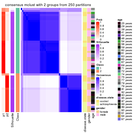
consensus_heatmap(res, k = 3)
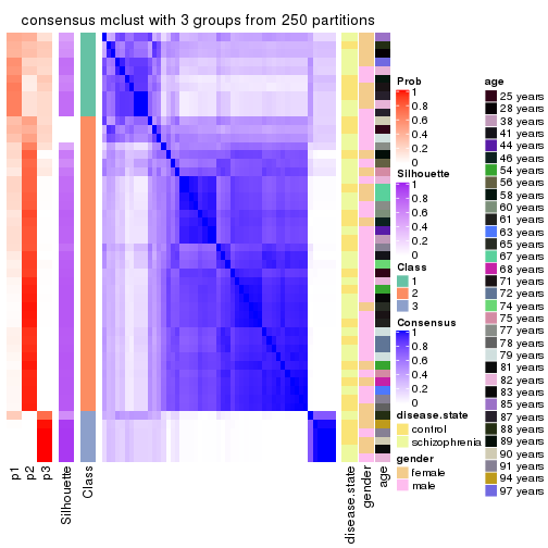
consensus_heatmap(res, k = 4)
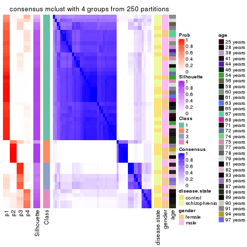
consensus_heatmap(res, k = 5)
consensus_heatmap(res, k = 6)
Heatmaps for the membership of samples in all partitions to see how consistent they are:
membership_heatmap(res, k = 2)
membership_heatmap(res, k = 3)
membership_heatmap(res, k = 4)
membership_heatmap(res, k = 5)
membership_heatmap(res, k = 6)
As soon as we have had the classes for columns, we can look for signatures which are significantly different between classes which can be candidate marks for certain classes. Following are the heatmaps for signatures.
Signature heatmaps where rows are scaled:
get_signatures(res, k = 2)
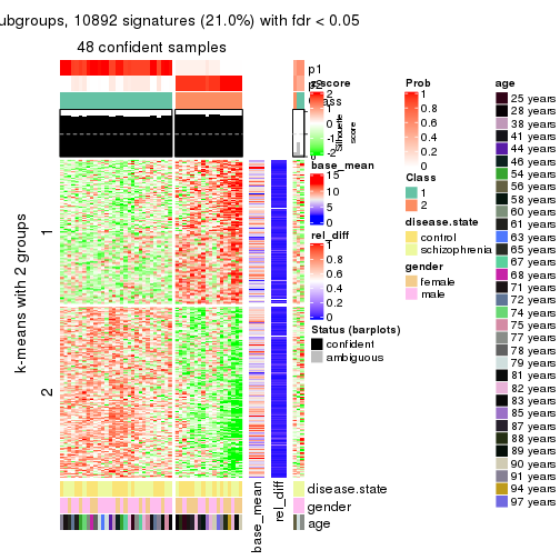
get_signatures(res, k = 3)
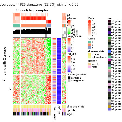
get_signatures(res, k = 4)
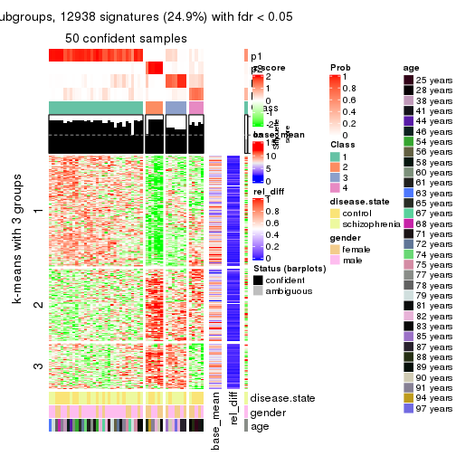
get_signatures(res, k = 5)
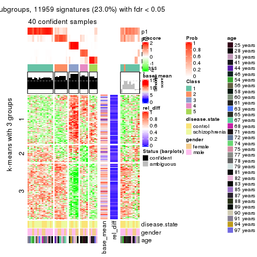
get_signatures(res, k = 6)
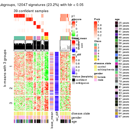
Signature heatmaps where rows are not scaled:
get_signatures(res, k = 2, scale_rows = FALSE)
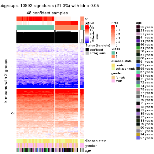
get_signatures(res, k = 3, scale_rows = FALSE)
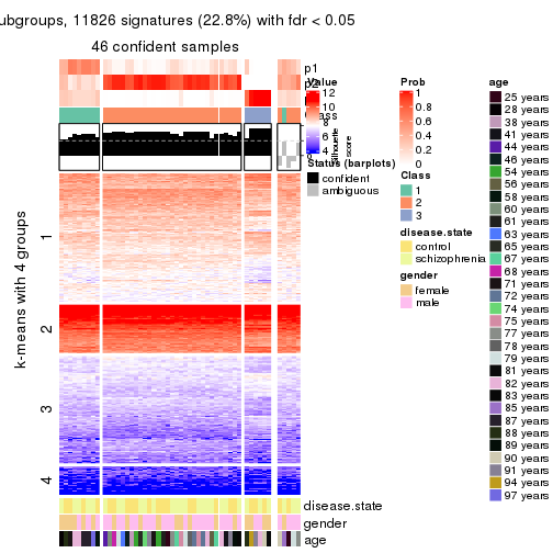
get_signatures(res, k = 4, scale_rows = FALSE)
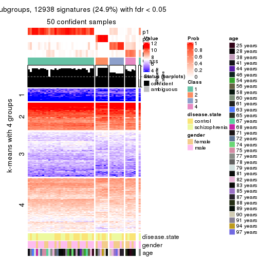
get_signatures(res, k = 5, scale_rows = FALSE)
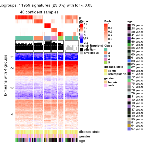
get_signatures(res, k = 6, scale_rows = FALSE)
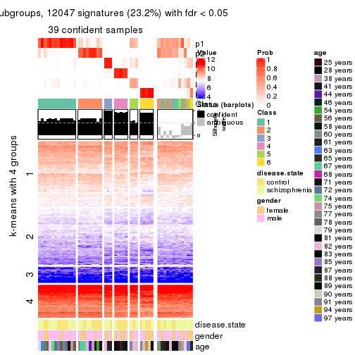
Compare the overlap of signatures from different k:
compare_signatures(res)
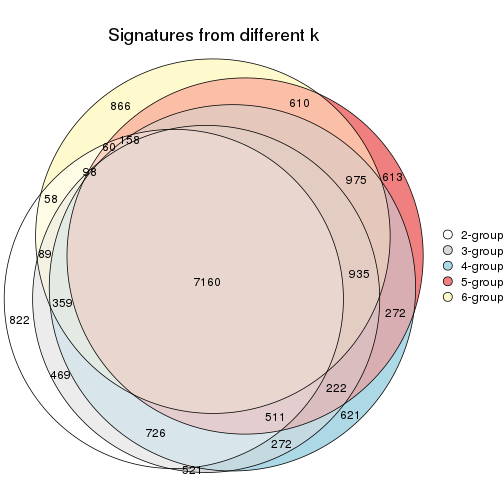
get_signature() returns a data frame invisibly. TO get the list of signatures, the function
call should be assigned to a variable explicitly. In following code, if plot argument is set
to FALSE, no heatmap is plotted while only the differential analysis is performed.
# code only for demonstration
tb = get_signature(res, k = ..., plot = FALSE)
An example of the output of tb is:
#> which_row fdr mean_1 mean_2 scaled_mean_1 scaled_mean_2 km
#> 1 38 0.042760348 8.373488 9.131774 -0.5533452 0.5164555 1
#> 2 40 0.018707592 7.106213 8.469186 -0.6173731 0.5762149 1
#> 3 55 0.019134737 10.221463 11.207825 -0.6159697 0.5749050 1
#> 4 59 0.006059896 5.921854 7.869574 -0.6899429 0.6439467 1
#> 5 60 0.018055526 8.928898 10.211722 -0.6204761 0.5791110 1
#> 6 98 0.009384629 15.714769 14.887706 0.6635654 -0.6193277 2
...
The columns in tb are:
which_row: row indices corresponding to the input matrix.fdr: FDR for the differential test. mean_x: The mean value in group x.scaled_mean_x: The mean value in group x after rows are scaled.km: Row groups if k-means clustering is applied to rows.UMAP plot which shows how samples are separated.
dimension_reduction(res, k = 2, method = "UMAP")
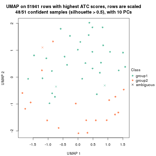
dimension_reduction(res, k = 3, method = "UMAP")
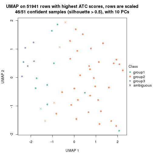
dimension_reduction(res, k = 4, method = "UMAP")
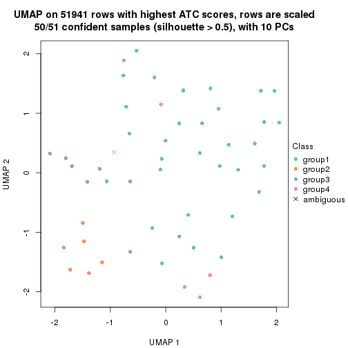
dimension_reduction(res, k = 5, method = "UMAP")
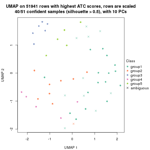
dimension_reduction(res, k = 6, method = "UMAP")
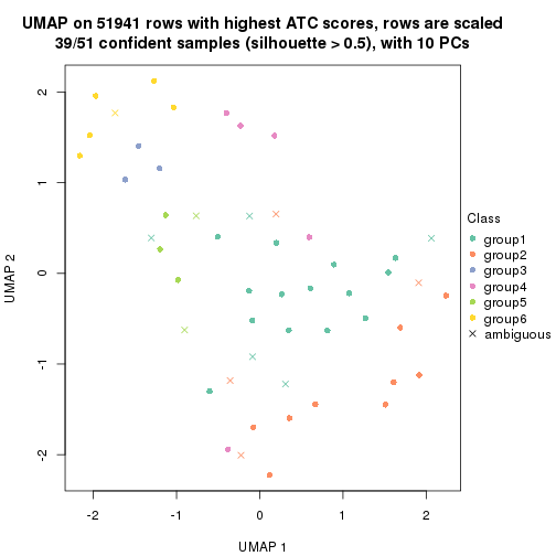
Following heatmap shows how subgroups are split when increasing k:
collect_classes(res)
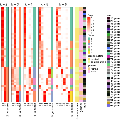
Test correlation between subgroups and known annotations. If the known annotation is numeric, one-way ANOVA test is applied, and if the known annotation is discrete, chi-squared contingency table test is applied.
test_to_known_factors(res)
#> n disease.state(p) gender(p) age(p) k
#> ATC:mclust 48 1.000 0.0696 0.254 2
#> ATC:mclust 46 0.973 0.0522 0.470 3
#> ATC:mclust 50 0.349 0.1480 0.429 4
#> ATC:mclust 40 0.367 0.3113 0.128 5
#> ATC:mclust 39 0.694 0.4385 0.272 6
If matrix rows can be associated to genes, consider to use functional_enrichment(res,
...) to perform function enrichment for the signature genes. See this vignette for more detailed explanations.
The object with results only for a single top-value method and a single partition method can be extracted as:
res = res_list["ATC", "NMF"]
# you can also extract it by
# res = res_list["ATC:NMF"]
A summary of res and all the functions that can be applied to it:
res
#> A 'ConsensusPartition' object with k = 2, 3, 4, 5, 6.
#> On a matrix with 51941 rows and 51 columns.
#> Top rows (1000, 2000, 3000, 4000, 5000) are extracted by 'ATC' method.
#> Subgroups are detected by 'NMF' method.
#> Performed in total 1250 partitions by row resampling.
#> Best k for subgroups seems to be 3.
#>
#> Following methods can be applied to this 'ConsensusPartition' object:
#> [1] "cola_report" "collect_classes" "collect_plots"
#> [4] "collect_stats" "colnames" "compare_signatures"
#> [7] "consensus_heatmap" "dimension_reduction" "functional_enrichment"
#> [10] "get_anno_col" "get_anno" "get_classes"
#> [13] "get_consensus" "get_matrix" "get_membership"
#> [16] "get_param" "get_signatures" "get_stats"
#> [19] "is_best_k" "is_stable_k" "membership_heatmap"
#> [22] "ncol" "nrow" "plot_ecdf"
#> [25] "rownames" "select_partition_number" "show"
#> [28] "suggest_best_k" "test_to_known_factors"
collect_plots() function collects all the plots made from res for all k (number of partitions)
into one single page to provide an easy and fast comparison between different k.
collect_plots(res)
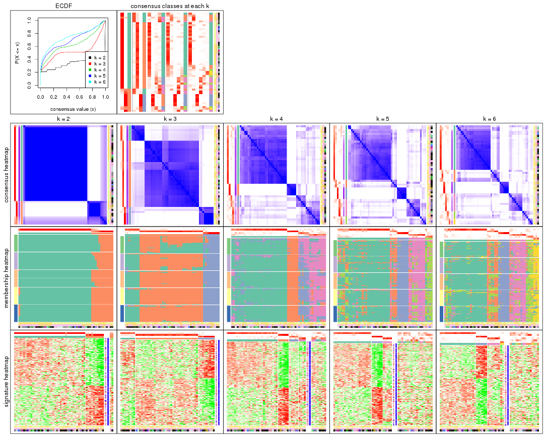
The plots are:
k and the heatmap of
predicted classes for each k.k.k.k.All the plots in panels can be made by individual functions and they are plotted later in this section.
select_partition_number() produces several plots showing different
statistics for choosing “optimized” k. There are following statistics:
k;k, the area increased is defined as \(A_k - A_{k-1}\).The detailed explanations of these statistics can be found in the cola vignette.
Generally speaking, lower PAC score, higher mean silhouette score or higher
concordance corresponds to better partition. Rand index and Jaccard index
measure how similar the current partition is compared to partition with k-1.
If they are too similar, we won't accept k is better than k-1.
select_partition_number(res)
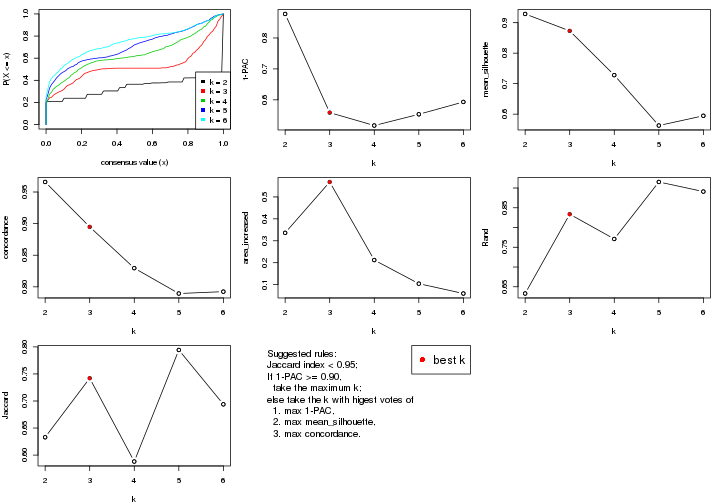
The numeric values for all these statistics can be obtained by get_stats().
get_stats(res)
#> k 1-PAC mean_silhouette concordance area_increased Rand Jaccard
#> 2 2 0.878 0.929 0.966 0.3362 0.633 0.633
#> 3 3 0.559 0.873 0.895 0.5682 0.834 0.742
#> 4 4 0.517 0.728 0.830 0.2120 0.771 0.588
#> 5 5 0.553 0.563 0.789 0.1044 0.915 0.794
#> 6 6 0.593 0.595 0.792 0.0594 0.891 0.694
suggest_best_k() suggests the best \(k\) based on these statistics. The rules are as follows:
suggest_best_k(res)
#> [1] 3
Following shows the table of the partitions (You need to click the show/hide
code output link to see it). The membership matrix (columns with name p*)
is inferred by
clue::cl_consensus()
function with the SE method. Basically the value in the membership matrix
represents the probability to belong to a certain group. The finall class
label for an item is determined with the group with highest probability it
belongs to.
In get_classes() function, the entropy is calculated from the membership
matrix and the silhouette score is calculated from the consensus matrix.
cbind(get_classes(res, k = 2), get_membership(res, k = 2))
#> class entropy silhouette p1 p2
#> GSM439800 1 0.0000 0.993 1.000 0.000
#> GSM439790 1 0.0000 0.993 1.000 0.000
#> GSM439827 1 0.0000 0.993 1.000 0.000
#> GSM439811 1 0.0000 0.993 1.000 0.000
#> GSM439795 2 0.0000 0.859 0.000 1.000
#> GSM439805 2 0.7674 0.735 0.224 0.776
#> GSM439781 1 0.0000 0.993 1.000 0.000
#> GSM439807 2 0.0000 0.859 0.000 1.000
#> GSM439820 2 0.9044 0.624 0.320 0.680
#> GSM439784 1 0.0000 0.993 1.000 0.000
#> GSM439824 1 0.0000 0.993 1.000 0.000
#> GSM439794 1 0.0000 0.993 1.000 0.000
#> GSM439809 1 0.0000 0.993 1.000 0.000
#> GSM439785 1 0.0000 0.993 1.000 0.000
#> GSM439803 1 0.0000 0.993 1.000 0.000
#> GSM439778 1 0.0000 0.993 1.000 0.000
#> GSM439791 1 0.0000 0.993 1.000 0.000
#> GSM439786 1 0.0000 0.993 1.000 0.000
#> GSM439828 1 0.0000 0.993 1.000 0.000
#> GSM439806 1 0.0000 0.993 1.000 0.000
#> GSM439815 1 0.0000 0.993 1.000 0.000
#> GSM439817 1 0.0000 0.993 1.000 0.000
#> GSM439796 1 0.0000 0.993 1.000 0.000
#> GSM439798 2 0.9922 0.366 0.448 0.552
#> GSM439821 2 0.0000 0.859 0.000 1.000
#> GSM439823 1 0.0000 0.993 1.000 0.000
#> GSM439813 1 0.0000 0.993 1.000 0.000
#> GSM439801 2 0.0000 0.859 0.000 1.000
#> GSM439810 1 0.0000 0.993 1.000 0.000
#> GSM439783 1 0.0000 0.993 1.000 0.000
#> GSM439826 1 0.0000 0.993 1.000 0.000
#> GSM439812 1 0.0000 0.993 1.000 0.000
#> GSM439818 1 0.7815 0.626 0.768 0.232
#> GSM439792 1 0.0000 0.993 1.000 0.000
#> GSM439802 2 0.4690 0.821 0.100 0.900
#> GSM439825 1 0.0000 0.993 1.000 0.000
#> GSM439780 1 0.0000 0.993 1.000 0.000
#> GSM439787 2 0.0000 0.859 0.000 1.000
#> GSM439808 2 0.0000 0.859 0.000 1.000
#> GSM439804 1 0.0000 0.993 1.000 0.000
#> GSM439822 1 0.0000 0.993 1.000 0.000
#> GSM439816 1 0.0000 0.993 1.000 0.000
#> GSM439789 1 0.0000 0.993 1.000 0.000
#> GSM439799 2 0.9775 0.457 0.412 0.588
#> GSM439814 1 0.0000 0.993 1.000 0.000
#> GSM439782 1 0.0000 0.993 1.000 0.000
#> GSM439779 1 0.0000 0.993 1.000 0.000
#> GSM439793 1 0.0376 0.988 0.996 0.004
#> GSM439788 1 0.0000 0.993 1.000 0.000
#> GSM439797 1 0.0000 0.993 1.000 0.000
#> GSM439819 2 0.0000 0.859 0.000 1.000
cbind(get_classes(res, k = 3), get_membership(res, k = 3))
#> class entropy silhouette p1 p2 p3
#> GSM439800 1 0.3686 0.929 0.860 0.140 0.000
#> GSM439790 2 0.1163 0.904 0.028 0.972 0.000
#> GSM439827 2 0.3482 0.853 0.128 0.872 0.000
#> GSM439811 2 0.3551 0.850 0.132 0.868 0.000
#> GSM439795 3 0.0000 0.910 0.000 0.000 1.000
#> GSM439805 1 0.5582 0.861 0.812 0.088 0.100
#> GSM439781 2 0.4805 0.812 0.176 0.812 0.012
#> GSM439807 3 0.0000 0.910 0.000 0.000 1.000
#> GSM439820 3 0.3539 0.803 0.012 0.100 0.888
#> GSM439784 2 0.2711 0.891 0.088 0.912 0.000
#> GSM439824 2 0.2711 0.875 0.088 0.912 0.000
#> GSM439794 1 0.3686 0.929 0.860 0.140 0.000
#> GSM439809 2 0.1643 0.902 0.044 0.956 0.000
#> GSM439785 2 0.1031 0.904 0.024 0.976 0.000
#> GSM439803 2 0.3816 0.842 0.148 0.852 0.000
#> GSM439778 2 0.4750 0.757 0.216 0.784 0.000
#> GSM439791 2 0.3038 0.869 0.104 0.896 0.000
#> GSM439786 2 0.1031 0.899 0.024 0.976 0.000
#> GSM439828 2 0.2448 0.893 0.076 0.924 0.000
#> GSM439806 2 0.2878 0.873 0.096 0.904 0.000
#> GSM439815 2 0.2165 0.897 0.064 0.936 0.000
#> GSM439817 2 0.1163 0.904 0.028 0.972 0.000
#> GSM439796 2 0.2878 0.884 0.096 0.904 0.000
#> GSM439798 3 0.5012 0.650 0.008 0.204 0.788
#> GSM439821 3 0.0000 0.910 0.000 0.000 1.000
#> GSM439823 2 0.2356 0.894 0.072 0.928 0.000
#> GSM439813 2 0.3551 0.849 0.132 0.868 0.000
#> GSM439801 3 0.4702 0.711 0.212 0.000 0.788
#> GSM439810 2 0.2878 0.872 0.096 0.904 0.000
#> GSM439783 2 0.2959 0.881 0.100 0.900 0.000
#> GSM439826 2 0.1163 0.905 0.028 0.972 0.000
#> GSM439812 2 0.0592 0.901 0.012 0.988 0.000
#> GSM439818 1 0.4139 0.928 0.860 0.124 0.016
#> GSM439792 2 0.2356 0.883 0.072 0.928 0.000
#> GSM439802 1 0.6208 0.787 0.772 0.076 0.152
#> GSM439825 1 0.3686 0.929 0.860 0.140 0.000
#> GSM439780 2 0.1643 0.902 0.044 0.956 0.000
#> GSM439787 3 0.0000 0.910 0.000 0.000 1.000
#> GSM439808 3 0.0000 0.910 0.000 0.000 1.000
#> GSM439804 2 0.3267 0.871 0.116 0.884 0.000
#> GSM439822 1 0.4178 0.891 0.828 0.172 0.000
#> GSM439816 2 0.2796 0.873 0.092 0.908 0.000
#> GSM439789 2 0.1163 0.904 0.028 0.972 0.000
#> GSM439799 1 0.4413 0.916 0.860 0.104 0.036
#> GSM439814 2 0.3038 0.867 0.104 0.896 0.000
#> GSM439782 2 0.4178 0.817 0.172 0.828 0.000
#> GSM439779 2 0.2711 0.887 0.088 0.912 0.000
#> GSM439793 2 0.4099 0.837 0.140 0.852 0.008
#> GSM439788 2 0.3116 0.876 0.108 0.892 0.000
#> GSM439797 2 0.0592 0.903 0.012 0.988 0.000
#> GSM439819 3 0.0000 0.910 0.000 0.000 1.000
cbind(get_classes(res, k = 4), get_membership(res, k = 4))
#> class entropy silhouette p1 p2 p3 p4
#> GSM439800 1 0.5536 0.483 0.592 0.000 0.024 0.384
#> GSM439790 1 0.1510 0.868 0.956 0.000 0.028 0.016
#> GSM439827 1 0.2197 0.851 0.916 0.000 0.080 0.004
#> GSM439811 1 0.4877 0.621 0.664 0.000 0.328 0.008
#> GSM439795 2 0.0000 0.970 0.000 1.000 0.000 0.000
#> GSM439805 4 0.4920 0.545 0.000 0.052 0.192 0.756
#> GSM439781 3 0.6713 0.540 0.092 0.012 0.612 0.284
#> GSM439807 2 0.2334 0.907 0.000 0.908 0.088 0.004
#> GSM439820 3 0.6484 0.518 0.004 0.232 0.644 0.120
#> GSM439784 1 0.4992 0.747 0.772 0.000 0.096 0.132
#> GSM439824 1 0.0804 0.869 0.980 0.000 0.012 0.008
#> GSM439794 4 0.1913 0.611 0.040 0.000 0.020 0.940
#> GSM439809 1 0.2413 0.860 0.916 0.000 0.064 0.020
#> GSM439785 1 0.0657 0.869 0.984 0.000 0.012 0.004
#> GSM439803 4 0.5457 0.462 0.184 0.000 0.088 0.728
#> GSM439778 4 0.6194 0.441 0.132 0.000 0.200 0.668
#> GSM439791 1 0.2867 0.836 0.884 0.000 0.104 0.012
#> GSM439786 1 0.4540 0.713 0.772 0.000 0.196 0.032
#> GSM439828 1 0.3687 0.840 0.856 0.000 0.080 0.064
#> GSM439806 1 0.1284 0.867 0.964 0.000 0.024 0.012
#> GSM439815 1 0.6398 0.314 0.576 0.000 0.344 0.080
#> GSM439817 1 0.3080 0.846 0.880 0.000 0.096 0.024
#> GSM439796 1 0.2179 0.863 0.924 0.000 0.012 0.064
#> GSM439798 3 0.5397 0.519 0.012 0.232 0.720 0.036
#> GSM439821 2 0.0000 0.970 0.000 1.000 0.000 0.000
#> GSM439823 1 0.3754 0.837 0.852 0.000 0.064 0.084
#> GSM439813 1 0.1767 0.861 0.944 0.000 0.044 0.012
#> GSM439801 4 0.6548 0.445 0.000 0.188 0.176 0.636
#> GSM439810 1 0.0657 0.869 0.984 0.000 0.004 0.012
#> GSM439783 1 0.2376 0.864 0.916 0.000 0.016 0.068
#> GSM439826 1 0.2586 0.863 0.912 0.000 0.048 0.040
#> GSM439812 1 0.1545 0.866 0.952 0.000 0.040 0.008
#> GSM439818 4 0.6751 0.354 0.036 0.276 0.060 0.628
#> GSM439792 1 0.2179 0.859 0.924 0.000 0.064 0.012
#> GSM439802 4 0.5185 0.541 0.000 0.076 0.176 0.748
#> GSM439825 4 0.4907 0.450 0.176 0.000 0.060 0.764
#> GSM439780 1 0.4728 0.687 0.752 0.000 0.216 0.032
#> GSM439787 2 0.0000 0.970 0.000 1.000 0.000 0.000
#> GSM439808 2 0.1302 0.953 0.000 0.956 0.044 0.000
#> GSM439804 1 0.2376 0.863 0.916 0.000 0.016 0.068
#> GSM439822 1 0.5772 0.639 0.672 0.000 0.068 0.260
#> GSM439816 1 0.0672 0.869 0.984 0.000 0.008 0.008
#> GSM439789 1 0.1109 0.869 0.968 0.000 0.004 0.028
#> GSM439799 4 0.1593 0.596 0.016 0.004 0.024 0.956
#> GSM439814 1 0.0672 0.868 0.984 0.000 0.008 0.008
#> GSM439782 1 0.3547 0.831 0.840 0.000 0.016 0.144
#> GSM439779 3 0.6685 0.549 0.160 0.000 0.616 0.224
#> GSM439793 3 0.3679 0.580 0.140 0.016 0.840 0.004
#> GSM439788 3 0.6926 0.336 0.112 0.000 0.496 0.392
#> GSM439797 1 0.3529 0.814 0.836 0.000 0.152 0.012
#> GSM439819 2 0.0469 0.962 0.000 0.988 0.012 0.000
cbind(get_classes(res, k = 5), get_membership(res, k = 5))
#> class entropy silhouette p1 p2 p3 p4 p5
#> GSM439800 1 0.5041 0.5789 0.732 0.168 0.004 0.084 0.012
#> GSM439790 1 0.1885 0.7567 0.936 0.032 0.000 0.020 0.012
#> GSM439827 1 0.6054 0.3897 0.596 0.200 0.000 0.004 0.200
#> GSM439811 5 0.6550 -0.1962 0.424 0.108 0.000 0.024 0.444
#> GSM439795 3 0.0000 0.9771 0.000 0.000 1.000 0.000 0.000
#> GSM439805 4 0.0798 0.7084 0.000 0.008 0.016 0.976 0.000
#> GSM439781 4 0.4674 0.4624 0.024 0.004 0.000 0.656 0.316
#> GSM439807 3 0.0960 0.9665 0.000 0.004 0.972 0.008 0.016
#> GSM439820 5 0.5103 0.4174 0.000 0.036 0.160 0.068 0.736
#> GSM439784 1 0.7138 0.2994 0.544 0.148 0.000 0.076 0.232
#> GSM439824 1 0.1560 0.7612 0.948 0.028 0.000 0.004 0.020
#> GSM439794 4 0.5432 0.3199 0.056 0.312 0.000 0.620 0.012
#> GSM439809 1 0.3812 0.7259 0.840 0.064 0.000 0.044 0.052
#> GSM439785 1 0.1329 0.7591 0.956 0.032 0.000 0.004 0.008
#> GSM439803 4 0.5397 0.4508 0.152 0.152 0.000 0.688 0.008
#> GSM439778 4 0.1638 0.6949 0.064 0.004 0.000 0.932 0.000
#> GSM439791 1 0.3124 0.7165 0.840 0.008 0.000 0.008 0.144
#> GSM439786 1 0.6944 0.0579 0.452 0.276 0.000 0.012 0.260
#> GSM439828 1 0.5107 0.3371 0.596 0.356 0.000 0.000 0.048
#> GSM439806 1 0.1560 0.7613 0.948 0.028 0.000 0.004 0.020
#> GSM439815 1 0.7718 0.0739 0.456 0.084 0.000 0.232 0.228
#> GSM439817 1 0.6632 0.0161 0.456 0.364 0.000 0.008 0.172
#> GSM439796 1 0.1788 0.7573 0.932 0.056 0.000 0.004 0.008
#> GSM439798 5 0.6631 0.2363 0.000 0.036 0.172 0.212 0.580
#> GSM439821 3 0.0000 0.9771 0.000 0.000 1.000 0.000 0.000
#> GSM439823 1 0.4527 0.5389 0.696 0.272 0.000 0.004 0.028
#> GSM439813 1 0.2946 0.7148 0.868 0.044 0.000 0.000 0.088
#> GSM439801 4 0.2439 0.6608 0.000 0.000 0.120 0.876 0.004
#> GSM439810 1 0.0671 0.7624 0.980 0.004 0.000 0.000 0.016
#> GSM439783 1 0.1282 0.7615 0.952 0.044 0.000 0.004 0.000
#> GSM439826 1 0.3441 0.6902 0.824 0.148 0.000 0.004 0.024
#> GSM439812 1 0.2656 0.7472 0.896 0.064 0.000 0.012 0.028
#> GSM439818 2 0.5881 0.3515 0.040 0.688 0.184 0.076 0.012
#> GSM439792 1 0.1597 0.7614 0.948 0.008 0.000 0.020 0.024
#> GSM439802 4 0.0898 0.7081 0.000 0.008 0.020 0.972 0.000
#> GSM439825 2 0.4897 0.4465 0.156 0.728 0.000 0.112 0.004
#> GSM439780 1 0.6862 0.1262 0.492 0.232 0.000 0.016 0.260
#> GSM439787 3 0.0000 0.9771 0.000 0.000 1.000 0.000 0.000
#> GSM439808 3 0.1341 0.9427 0.000 0.000 0.944 0.000 0.056
#> GSM439804 1 0.1502 0.7590 0.940 0.056 0.000 0.004 0.000
#> GSM439822 2 0.4680 -0.0842 0.448 0.540 0.000 0.008 0.004
#> GSM439816 1 0.0854 0.7630 0.976 0.008 0.000 0.004 0.012
#> GSM439789 1 0.0932 0.7627 0.972 0.020 0.000 0.004 0.004
#> GSM439799 2 0.4889 -0.1935 0.004 0.504 0.000 0.476 0.016
#> GSM439814 1 0.1281 0.7622 0.956 0.032 0.000 0.000 0.012
#> GSM439782 1 0.2757 0.7432 0.888 0.072 0.000 0.032 0.008
#> GSM439779 4 0.5768 0.3345 0.084 0.008 0.000 0.580 0.328
#> GSM439793 5 0.4356 0.3850 0.032 0.008 0.020 0.152 0.788
#> GSM439788 4 0.3915 0.6266 0.024 0.012 0.000 0.792 0.172
#> GSM439797 1 0.3681 0.6824 0.820 0.008 0.000 0.136 0.036
#> GSM439819 3 0.0771 0.9619 0.000 0.020 0.976 0.000 0.004
cbind(get_classes(res, k = 6), get_membership(res, k = 6))
#> class entropy silhouette p1 p2 p3 p4 p5 p6
#> GSM439800 1 0.4002 0.7367 0.812 0.088 0.004 0.008 0.036 0.052
#> GSM439790 1 0.1788 0.8398 0.928 0.004 0.000 0.028 0.000 0.040
#> GSM439827 1 0.6270 -0.2798 0.404 0.312 0.000 0.000 0.276 0.008
#> GSM439811 5 0.5719 0.3058 0.136 0.212 0.000 0.024 0.620 0.008
#> GSM439795 3 0.0000 0.9352 0.000 0.000 1.000 0.000 0.000 0.000
#> GSM439805 4 0.0810 0.6771 0.000 0.008 0.004 0.976 0.004 0.008
#> GSM439781 4 0.4062 0.5562 0.000 0.012 0.000 0.724 0.236 0.028
#> GSM439807 3 0.1476 0.9204 0.000 0.012 0.948 0.008 0.028 0.004
#> GSM439820 5 0.5303 0.3098 0.000 0.108 0.028 0.052 0.720 0.092
#> GSM439784 5 0.7993 0.2436 0.244 0.188 0.000 0.176 0.364 0.028
#> GSM439824 1 0.0551 0.8417 0.984 0.004 0.000 0.000 0.008 0.004
#> GSM439794 4 0.7923 0.2684 0.140 0.248 0.000 0.424 0.124 0.064
#> GSM439809 1 0.4065 0.7201 0.784 0.012 0.000 0.128 0.068 0.008
#> GSM439785 1 0.1411 0.8375 0.936 0.000 0.000 0.004 0.000 0.060
#> GSM439803 4 0.6859 0.3691 0.220 0.088 0.000 0.560 0.076 0.056
#> GSM439778 4 0.2377 0.6517 0.076 0.008 0.000 0.892 0.024 0.000
#> GSM439791 1 0.3050 0.7949 0.856 0.004 0.000 0.016 0.096 0.028
#> GSM439786 6 0.2956 0.5758 0.080 0.004 0.000 0.004 0.052 0.860
#> GSM439828 2 0.5243 0.1125 0.456 0.460 0.000 0.000 0.080 0.004
#> GSM439806 1 0.1194 0.8384 0.956 0.000 0.000 0.008 0.032 0.004
#> GSM439815 1 0.6412 0.1544 0.504 0.040 0.000 0.292 0.160 0.004
#> GSM439817 2 0.5054 0.0462 0.092 0.572 0.000 0.000 0.336 0.000
#> GSM439796 1 0.1462 0.8363 0.936 0.008 0.000 0.000 0.000 0.056
#> GSM439798 6 0.6617 0.2560 0.000 0.004 0.064 0.136 0.316 0.480
#> GSM439821 3 0.0000 0.9352 0.000 0.000 1.000 0.000 0.000 0.000
#> GSM439823 1 0.4795 0.3344 0.628 0.312 0.000 0.000 0.044 0.016
#> GSM439813 1 0.2662 0.8135 0.884 0.004 0.000 0.008 0.048 0.056
#> GSM439801 4 0.2994 0.5690 0.000 0.000 0.208 0.788 0.004 0.000
#> GSM439810 1 0.0363 0.8427 0.988 0.000 0.000 0.000 0.000 0.012
#> GSM439783 1 0.0291 0.8439 0.992 0.004 0.000 0.000 0.004 0.000
#> GSM439826 1 0.3022 0.7537 0.848 0.112 0.000 0.000 0.020 0.020
#> GSM439812 1 0.2572 0.8145 0.896 0.016 0.000 0.024 0.052 0.012
#> GSM439818 2 0.2170 0.3520 0.024 0.920 0.020 0.016 0.020 0.000
#> GSM439792 1 0.1680 0.8348 0.940 0.004 0.000 0.012 0.024 0.020
#> GSM439802 4 0.1406 0.6773 0.000 0.016 0.020 0.952 0.004 0.008
#> GSM439825 2 0.1710 0.3552 0.020 0.940 0.000 0.020 0.012 0.008
#> GSM439780 6 0.4266 0.5329 0.172 0.004 0.000 0.000 0.088 0.736
#> GSM439787 3 0.0000 0.9352 0.000 0.000 1.000 0.000 0.000 0.000
#> GSM439808 3 0.3184 0.8299 0.000 0.016 0.836 0.000 0.120 0.028
#> GSM439804 1 0.1265 0.8399 0.948 0.008 0.000 0.000 0.000 0.044
#> GSM439822 2 0.4533 0.2804 0.380 0.588 0.000 0.000 0.016 0.016
#> GSM439816 1 0.0777 0.8416 0.972 0.004 0.000 0.000 0.000 0.024
#> GSM439789 1 0.1036 0.8441 0.964 0.000 0.000 0.004 0.008 0.024
#> GSM439799 2 0.6248 -0.0259 0.000 0.544 0.000 0.276 0.096 0.084
#> GSM439814 1 0.0551 0.8421 0.984 0.004 0.000 0.004 0.008 0.000
#> GSM439782 1 0.2138 0.8295 0.912 0.012 0.000 0.008 0.008 0.060
#> GSM439779 4 0.4819 0.5131 0.068 0.004 0.000 0.688 0.224 0.016
#> GSM439793 5 0.5045 0.1551 0.016 0.008 0.004 0.084 0.696 0.192
#> GSM439788 4 0.3183 0.6441 0.004 0.000 0.000 0.828 0.128 0.040
#> GSM439797 1 0.3698 0.7261 0.796 0.004 0.000 0.148 0.044 0.008
#> GSM439819 3 0.2070 0.8651 0.000 0.092 0.896 0.000 0.012 0.000
Heatmaps for the consensus matrix. It visualizes the probability of two samples to be in a same group.
consensus_heatmap(res, k = 2)
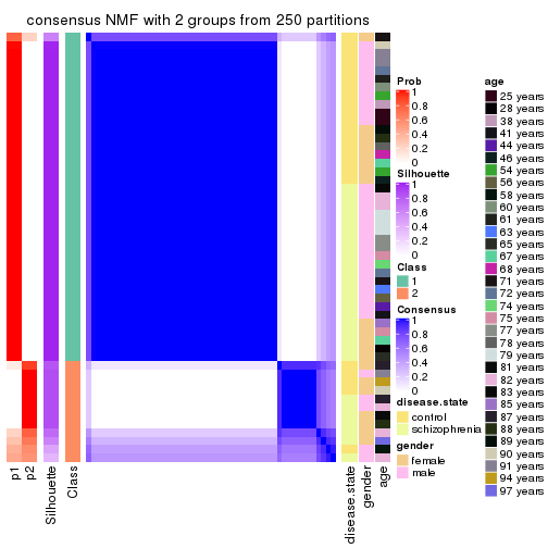
consensus_heatmap(res, k = 3)
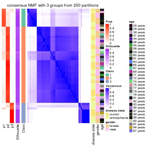
consensus_heatmap(res, k = 4)
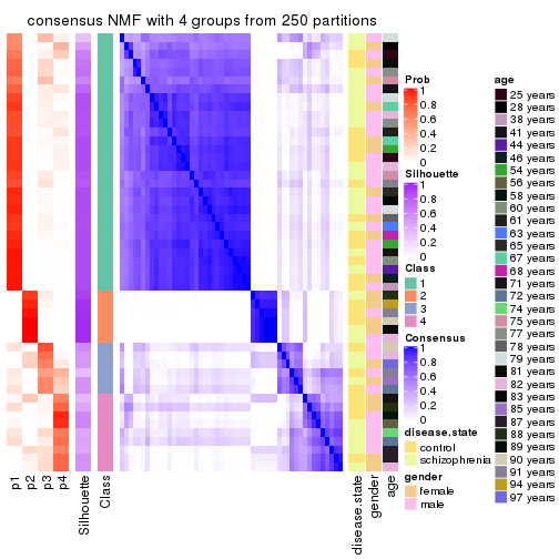
consensus_heatmap(res, k = 5)
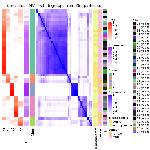
consensus_heatmap(res, k = 6)
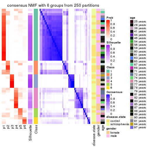
Heatmaps for the membership of samples in all partitions to see how consistent they are:
membership_heatmap(res, k = 2)
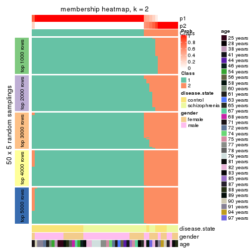
membership_heatmap(res, k = 3)
membership_heatmap(res, k = 4)
membership_heatmap(res, k = 5)
membership_heatmap(res, k = 6)
As soon as we have had the classes for columns, we can look for signatures which are significantly different between classes which can be candidate marks for certain classes. Following are the heatmaps for signatures.
Signature heatmaps where rows are scaled:
get_signatures(res, k = 2)
get_signatures(res, k = 3)
get_signatures(res, k = 4)
get_signatures(res, k = 5)
get_signatures(res, k = 6)
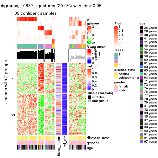
Signature heatmaps where rows are not scaled:
get_signatures(res, k = 2, scale_rows = FALSE)
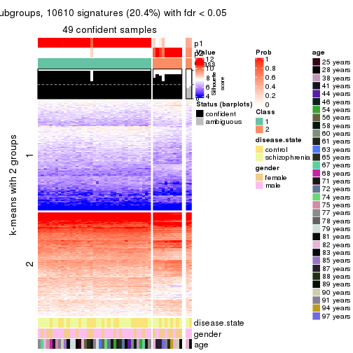
get_signatures(res, k = 3, scale_rows = FALSE)
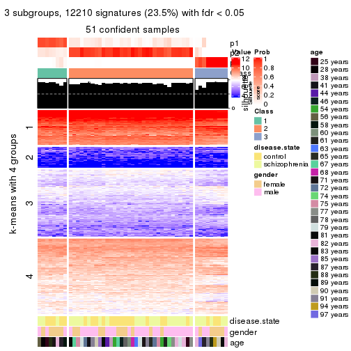
get_signatures(res, k = 4, scale_rows = FALSE)
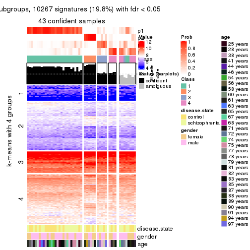
get_signatures(res, k = 5, scale_rows = FALSE)
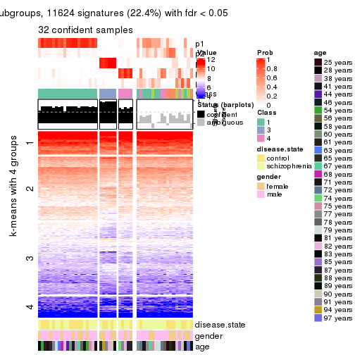
get_signatures(res, k = 6, scale_rows = FALSE)
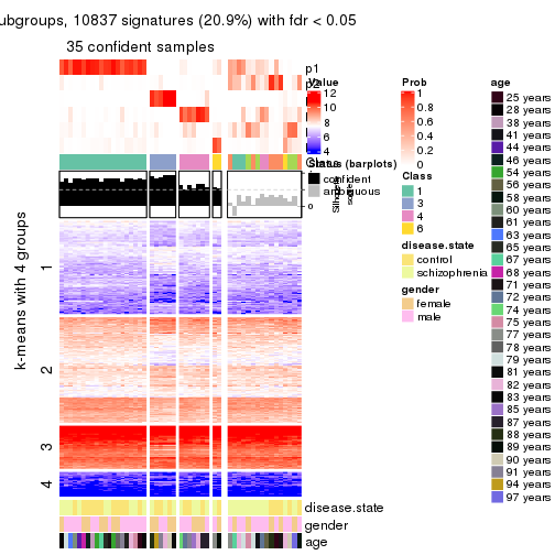
Compare the overlap of signatures from different k:
compare_signatures(res)
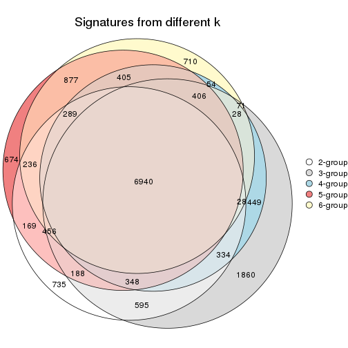
get_signature() returns a data frame invisibly. TO get the list of signatures, the function
call should be assigned to a variable explicitly. In following code, if plot argument is set
to FALSE, no heatmap is plotted while only the differential analysis is performed.
# code only for demonstration
tb = get_signature(res, k = ..., plot = FALSE)
An example of the output of tb is:
#> which_row fdr mean_1 mean_2 scaled_mean_1 scaled_mean_2 km
#> 1 38 0.042760348 8.373488 9.131774 -0.5533452 0.5164555 1
#> 2 40 0.018707592 7.106213 8.469186 -0.6173731 0.5762149 1
#> 3 55 0.019134737 10.221463 11.207825 -0.6159697 0.5749050 1
#> 4 59 0.006059896 5.921854 7.869574 -0.6899429 0.6439467 1
#> 5 60 0.018055526 8.928898 10.211722 -0.6204761 0.5791110 1
#> 6 98 0.009384629 15.714769 14.887706 0.6635654 -0.6193277 2
...
The columns in tb are:
which_row: row indices corresponding to the input matrix.fdr: FDR for the differential test. mean_x: The mean value in group x.scaled_mean_x: The mean value in group x after rows are scaled.km: Row groups if k-means clustering is applied to rows.UMAP plot which shows how samples are separated.
dimension_reduction(res, k = 2, method = "UMAP")
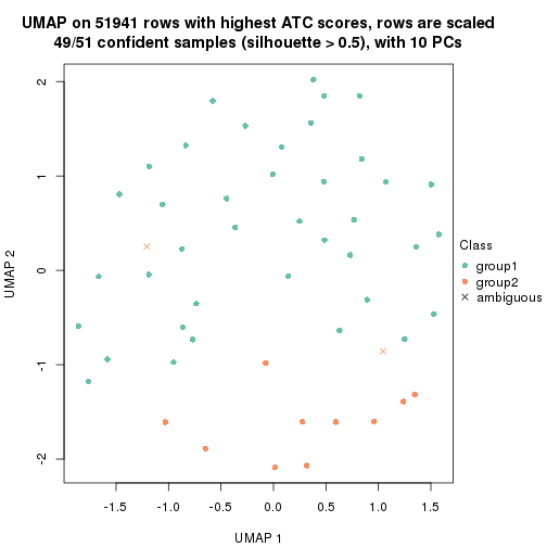
dimension_reduction(res, k = 3, method = "UMAP")
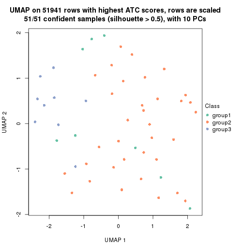
dimension_reduction(res, k = 4, method = "UMAP")
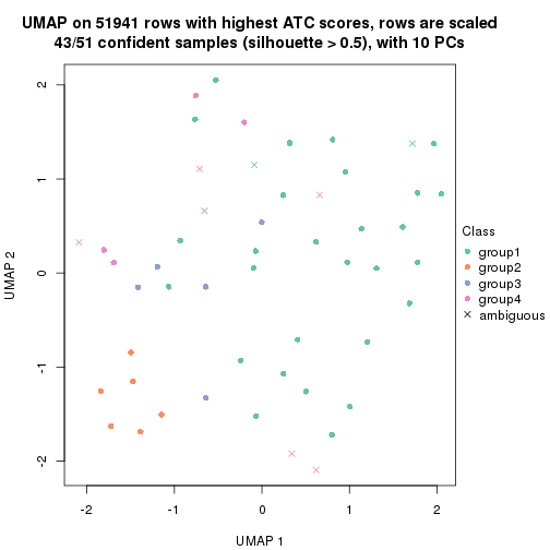
dimension_reduction(res, k = 5, method = "UMAP")
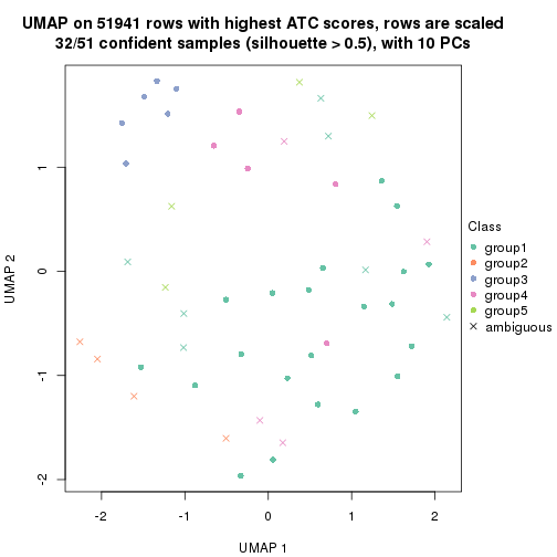
dimension_reduction(res, k = 6, method = "UMAP")
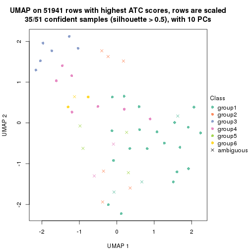
Following heatmap shows how subgroups are split when increasing k:
collect_classes(res)
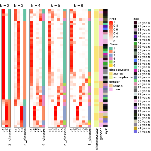
Test correlation between subgroups and known annotations. If the known annotation is numeric, one-way ANOVA test is applied, and if the known annotation is discrete, chi-squared contingency table test is applied.
test_to_known_factors(res)
#> n disease.state(p) gender(p) age(p) k
#> ATC:NMF 49 1.000 0.0811 0.389 2
#> ATC:NMF 51 0.474 0.1225 0.618 3
#> ATC:NMF 43 0.987 0.4451 0.374 4
#> ATC:NMF 32 0.884 0.3412 0.603 5
#> ATC:NMF 35 0.957 0.5861 0.355 6
If matrix rows can be associated to genes, consider to use functional_enrichment(res,
...) to perform function enrichment for the signature genes. See this vignette for more detailed explanations.
sessionInfo()
#> R version 3.6.0 (2019-04-26)
#> Platform: x86_64-pc-linux-gnu (64-bit)
#> Running under: CentOS Linux 7 (Core)
#>
#> Matrix products: default
#> BLAS: /usr/lib64/libblas.so.3.4.2
#> LAPACK: /usr/lib64/liblapack.so.3.4.2
#>
#> locale:
#> [1] LC_CTYPE=en_GB.UTF-8 LC_NUMERIC=C LC_TIME=en_GB.UTF-8
#> [4] LC_COLLATE=en_GB.UTF-8 LC_MONETARY=en_GB.UTF-8 LC_MESSAGES=en_GB.UTF-8
#> [7] LC_PAPER=en_GB.UTF-8 LC_NAME=C LC_ADDRESS=C
#> [10] LC_TELEPHONE=C LC_MEASUREMENT=en_GB.UTF-8 LC_IDENTIFICATION=C
#>
#> attached base packages:
#> [1] grid stats graphics grDevices utils datasets methods base
#>
#> other attached packages:
#> [1] genefilter_1.66.0 ComplexHeatmap_2.3.1 markdown_1.1 knitr_1.26
#> [5] GetoptLong_0.1.7 cola_1.3.2
#>
#> loaded via a namespace (and not attached):
#> [1] circlize_0.4.8 shape_1.4.4 xfun_0.11 slam_0.1-46
#> [5] lattice_0.20-38 splines_3.6.0 colorspace_1.4-1 vctrs_0.2.0
#> [9] stats4_3.6.0 blob_1.2.0 XML_3.98-1.20 survival_2.44-1.1
#> [13] rlang_0.4.2 pillar_1.4.2 DBI_1.0.0 BiocGenerics_0.30.0
#> [17] bit64_0.9-7 RColorBrewer_1.1-2 matrixStats_0.55.0 stringr_1.4.0
#> [21] GlobalOptions_0.1.1 evaluate_0.14 memoise_1.1.0 Biobase_2.44.0
#> [25] IRanges_2.18.3 parallel_3.6.0 AnnotationDbi_1.46.1 highr_0.8
#> [29] Rcpp_1.0.3 xtable_1.8-4 backports_1.1.5 S4Vectors_0.22.1
#> [33] annotate_1.62.0 skmeans_0.2-11 bit_1.1-14 microbenchmark_1.4-7
#> [37] brew_1.0-6 impute_1.58.0 rjson_0.2.20 png_0.1-7
#> [41] digest_0.6.23 stringi_1.4.3 polyclip_1.10-0 clue_0.3-57
#> [45] tools_3.6.0 bitops_1.0-6 magrittr_1.5 eulerr_6.0.0
#> [49] RCurl_1.95-4.12 RSQLite_2.1.4 tibble_2.1.3 cluster_2.1.0
#> [53] crayon_1.3.4 pkgconfig_2.0.3 zeallot_0.1.0 Matrix_1.2-17
#> [57] xml2_1.2.2 httr_1.4.1 R6_2.4.1 mclust_5.4.5
#> [61] compiler_3.6.0