
Date: 2019-12-25 20:41:45 CET, cola version: 1.3.2
Document is loading...
All available functions which can be applied to this res_list object:
res_list
#> A 'ConsensusPartitionList' object with 24 methods.
#>   On a matrix with 15834 rows and 54 columns.
#>   Top rows are extracted by 'SD, CV, MAD, ATC' methods.
#>   Subgroups are detected by 'hclust, kmeans, skmeans, pam, mclust, NMF' method.
#>   Number of partitions are tried for k = 2, 3, 4, 5, 6.
#>   Performed in total 30000 partitions by row resampling.
#>
#> Following methods can be applied to this 'ConsensusPartitionList' object:
#>  [1] "cola_report"           "collect_classes"       "collect_plots"         "collect_stats"
#>  [5] "colnames"              "functional_enrichment" "get_anno_col"          "get_anno"
#>  [9] "get_classes"           "get_matrix"            "get_membership"        "get_stats"
#> [13] "is_best_k"             "is_stable_k"           "ncol"                  "nrow"
#> [17] "rownames"              "show"                  "suggest_best_k"        "test_to_known_factors"
#> [21] "top_rows_heatmap"      "top_rows_overlap"
#>
#> You can get result for a single method by, e.g. object["SD", "hclust"] or object["SD:hclust"]
#> or a subset of methods by object[c("SD", "CV")], c("hclust", "kmeans")]
The call of run_all_consensus_partition_methods() was:
#> run_all_consensus_partition_methods(data = mat, mc.cores = 4, anno = anno)
Dimension of the input matrix:
mat = get_matrix(res_list)
dim(mat)
#> [1] 15834 54
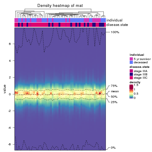
The density distribution for each sample is visualized as in one column in the following heatmap. The clustering is based on the distance which is the Kolmogorov-Smirnov statistic between two distributions.
library(ComplexHeatmap)
densityHeatmap(mat, top_annotation = HeatmapAnnotation(df = get_anno(res_list),
    col = get_anno_col(res_list)), ylab = "value", cluster_columns = TRUE, show_column_names = FALSE,
    mc.cores = 4)
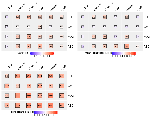
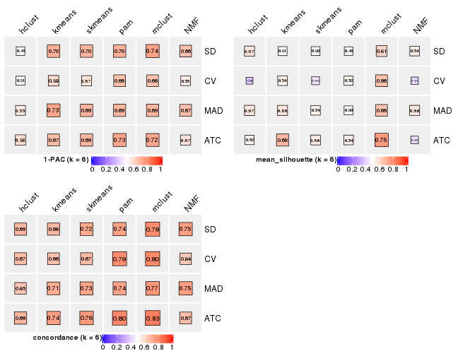
Folowing table shows the best k (number of partitions) for each combination
of top-value methods and partition methods. Clicking on the method name in
the table goes to the section for a single combination of methods.
The cola vignette explains the definition of the metrics used for determining the best number of partitions.
suggest_best_k(res_list)
| The best k | 1-PAC | Mean silhouette | Concordance | ||
|---|---|---|---|---|---|
| MAD:skmeans | 2 | 1.000 | 0.960 | 0.983 | ** |
| ATC:skmeans | 2 | 1.000 | 0.958 | 0.984 | ** |
| ATC:pam | 2 | 1.000 | 0.974 | 0.986 | ** |
| ATC:kmeans | 2 | 0.887 | 0.962 | 0.982 | |
| MAD:kmeans | 2 | 0.884 | 0.867 | 0.948 | |
| SD:skmeans | 2 | 0.851 | 0.923 | 0.968 | |
| ATC:NMF | 2 | 0.851 | 0.937 | 0.973 | |
| CV:skmeans | 2 | 0.752 | 0.878 | 0.948 | |
| MAD:pam | 2 | 0.714 | 0.862 | 0.938 | |
| SD:kmeans | 2 | 0.714 | 0.845 | 0.925 | |
| MAD:NMF | 2 | 0.677 | 0.856 | 0.939 | |
| CV:mclust | 6 | 0.658 | 0.660 | 0.801 | |
| CV:kmeans | 2 | 0.656 | 0.854 | 0.929 | |
| SD:NMF | 2 | 0.646 | 0.842 | 0.935 | |
| SD:mclust | 5 | 0.628 | 0.591 | 0.763 | |
| MAD:mclust | 5 | 0.620 | 0.621 | 0.799 | |
| CV:NMF | 2 | 0.618 | 0.847 | 0.934 | |
| MAD:hclust | 6 | 0.555 | 0.569 | 0.650 | |
| SD:pam | 2 | 0.547 | 0.853 | 0.928 | |
| ATC:mclust | 2 | 0.490 | 0.955 | 0.896 | |
| CV:hclust | 5 | 0.464 | 0.429 | 0.716 | |
| CV:pam | 2 | 0.451 | 0.685 | 0.823 | |
| ATC:hclust | 2 | 0.289 | 0.681 | 0.846 | |
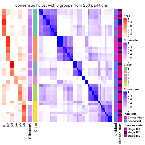
| SD:hclust | 2 | 0.094 | 0.588 | 0.751 |
**: 1-PAC > 0.95, *: 1-PAC > 0.9
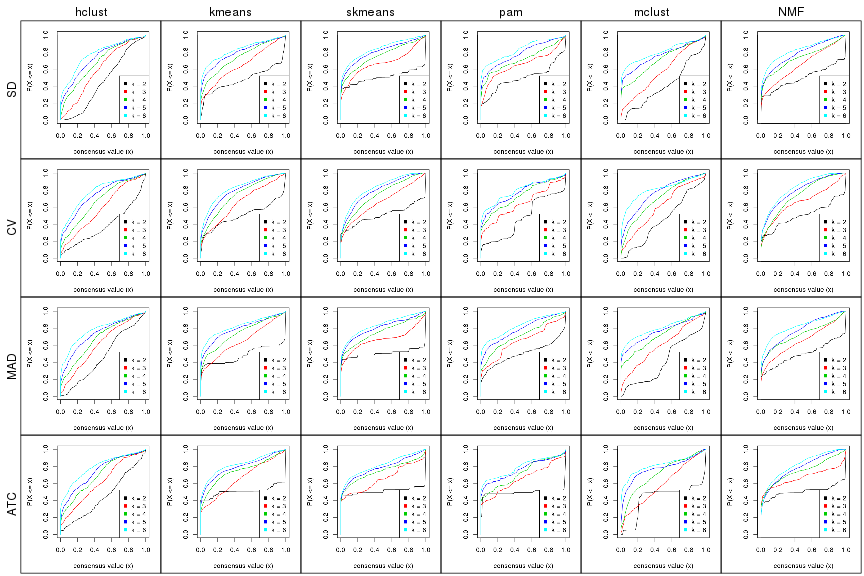
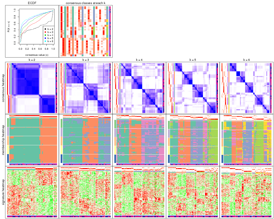
Cumulative distribution function curves of consensus matrix for all methods.
collect_plots(res_list, fun = plot_ecdf)
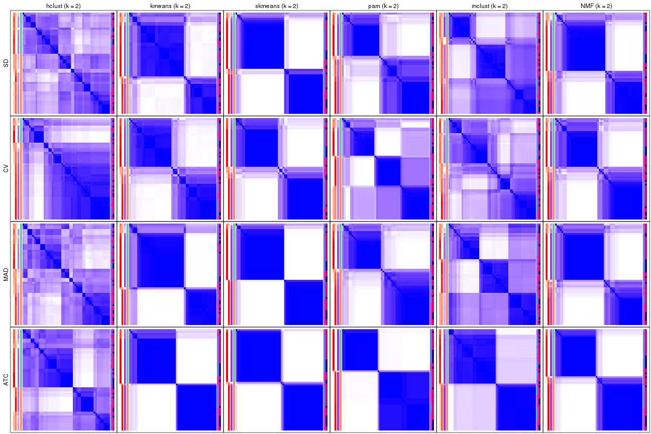
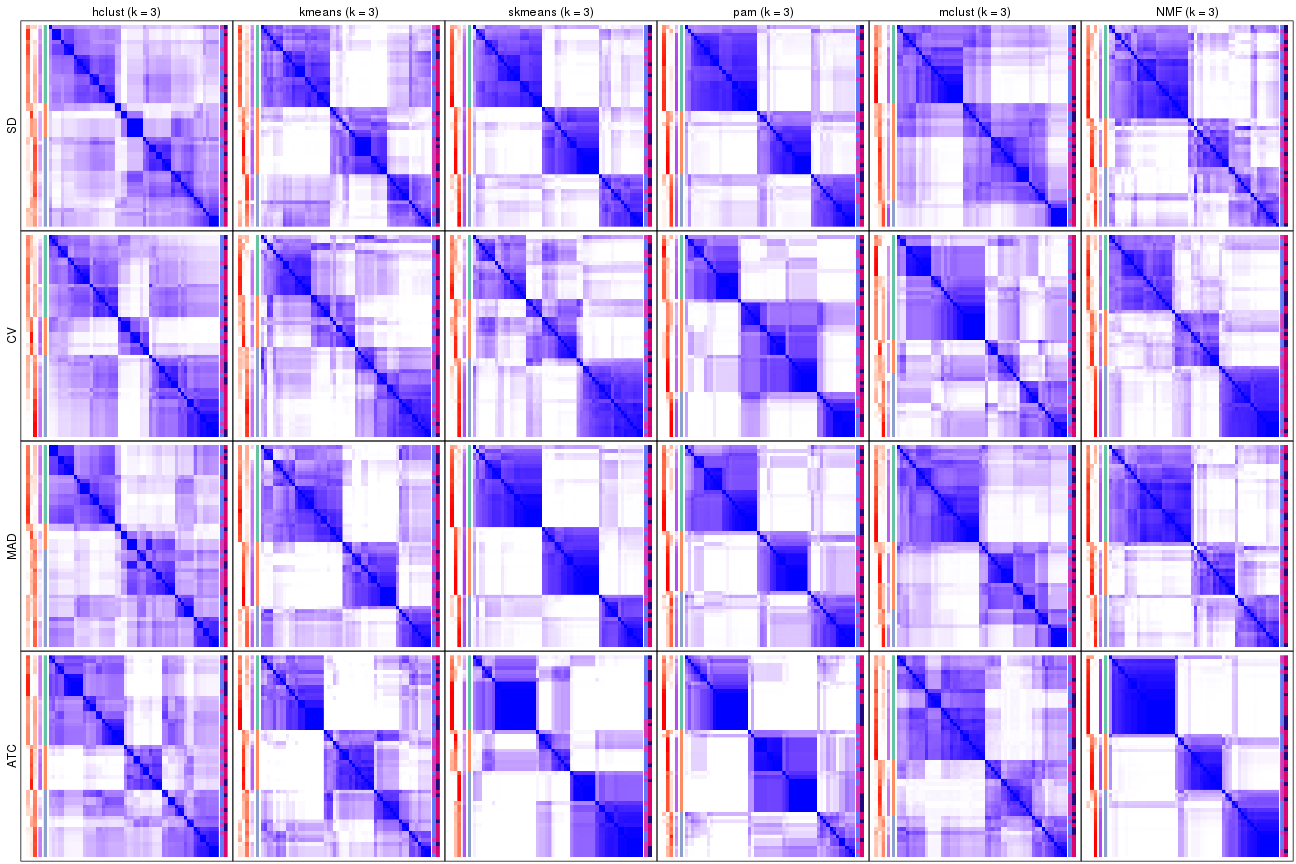
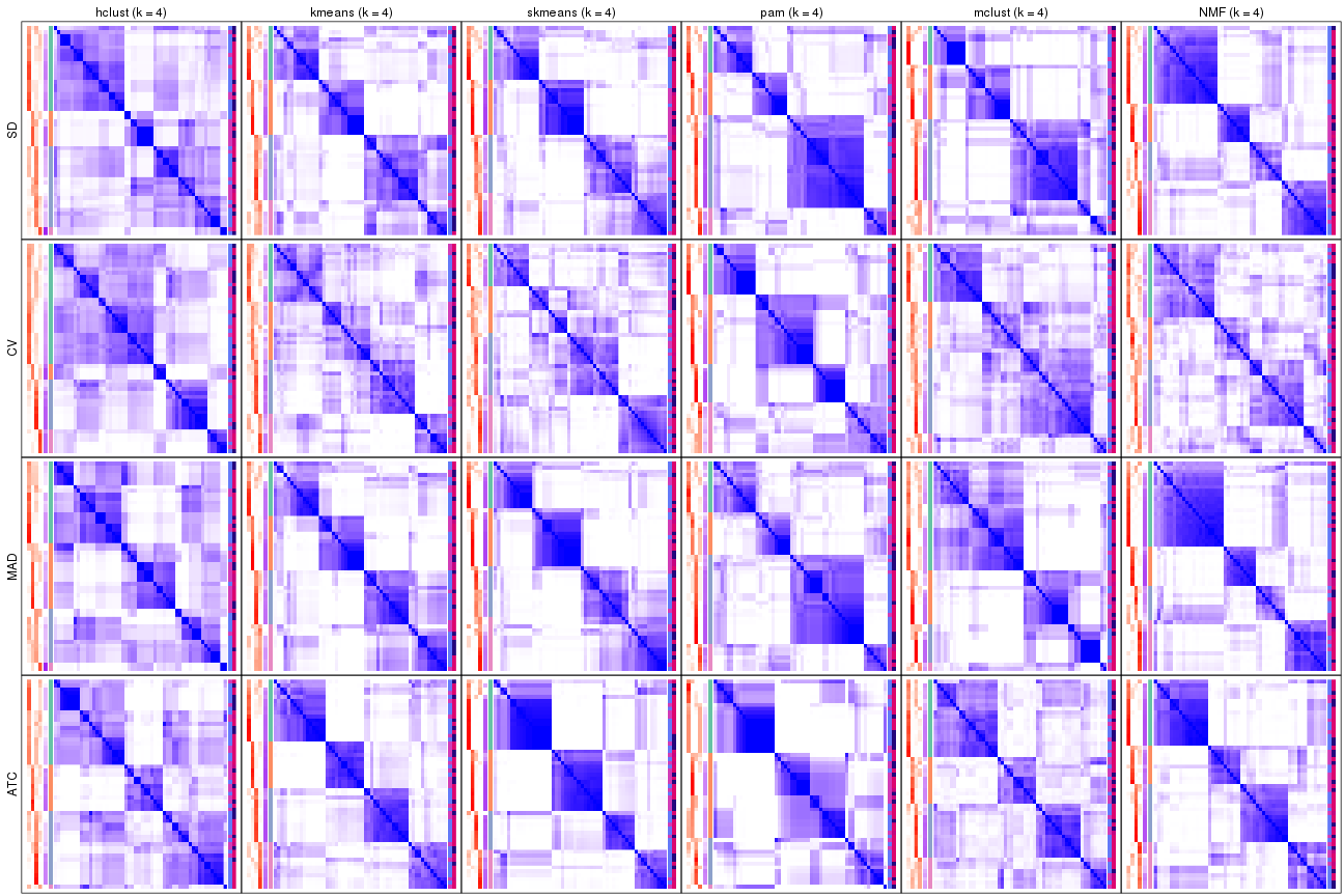
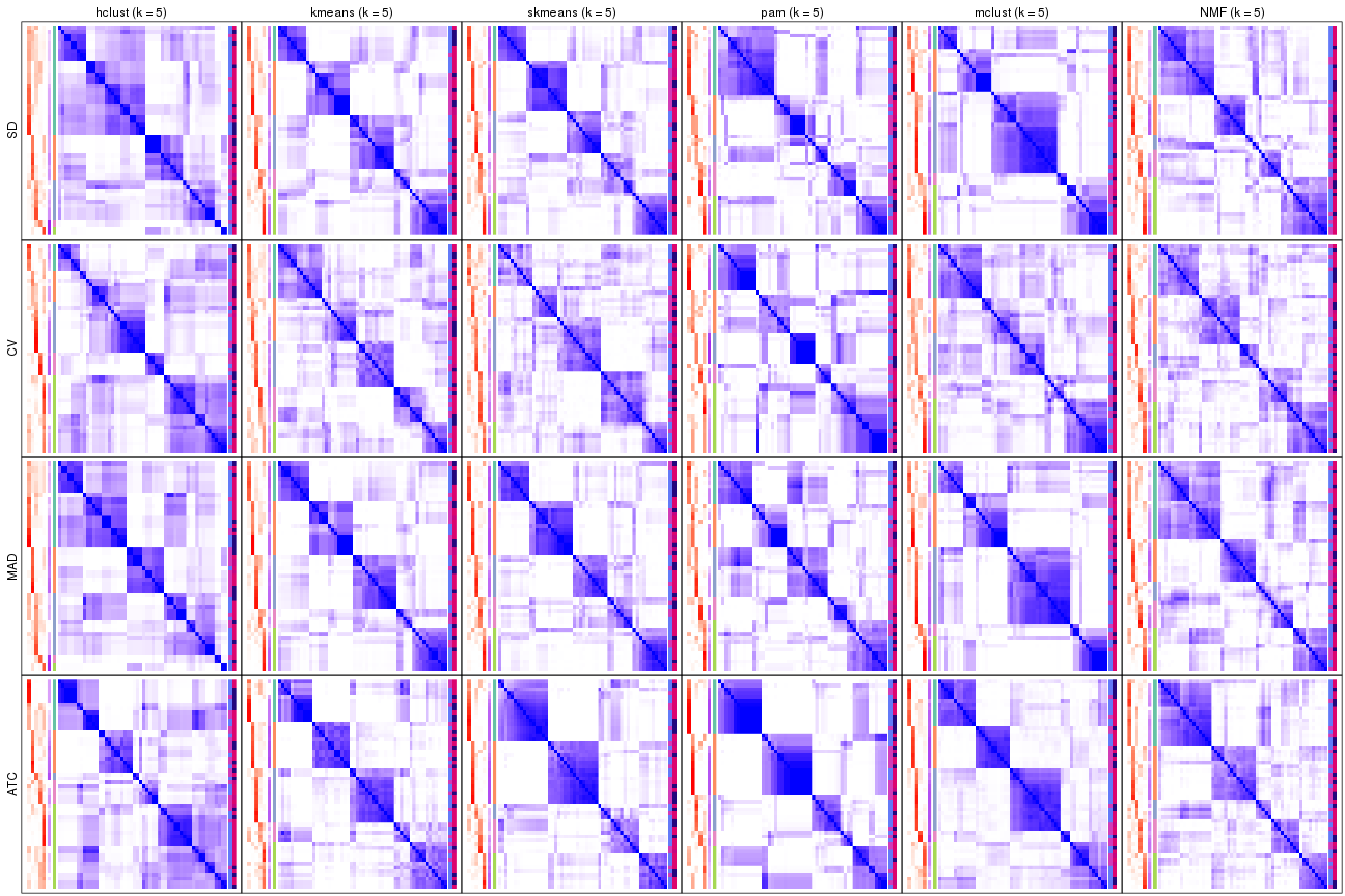
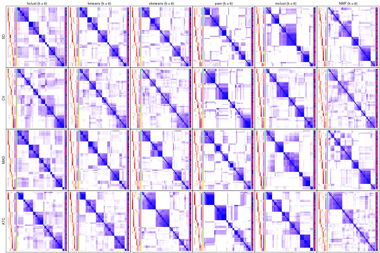
Consensus heatmaps for all methods. (What is a consensus heatmap?)
collect_plots(res_list, k = 2, fun = consensus_heatmap, mc.cores = 4)
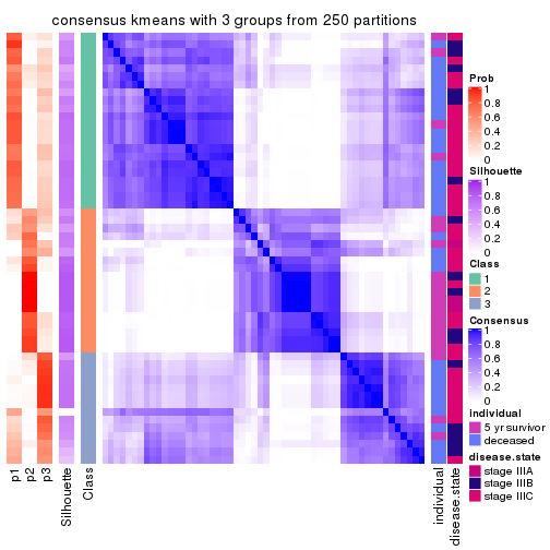
collect_plots(res_list, k = 3, fun = consensus_heatmap, mc.cores = 4)
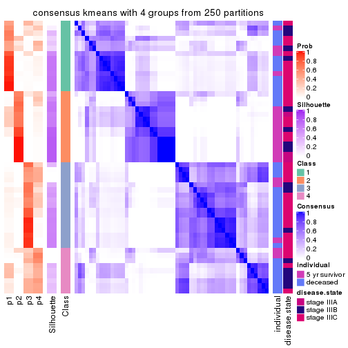
collect_plots(res_list, k = 4, fun = consensus_heatmap, mc.cores = 4)
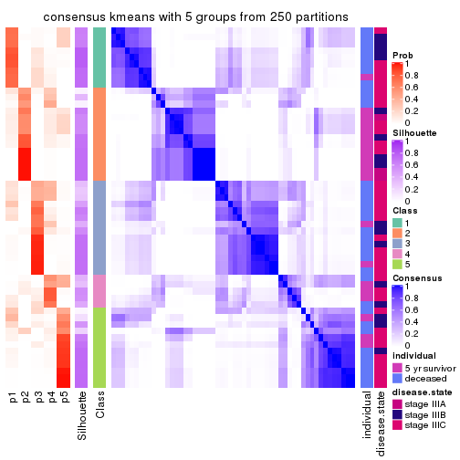
collect_plots(res_list, k = 5, fun = consensus_heatmap, mc.cores = 4)
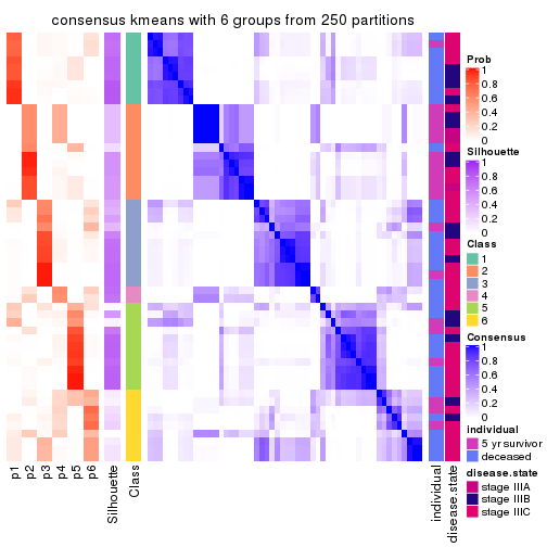
collect_plots(res_list, k = 6, fun = consensus_heatmap, mc.cores = 4)
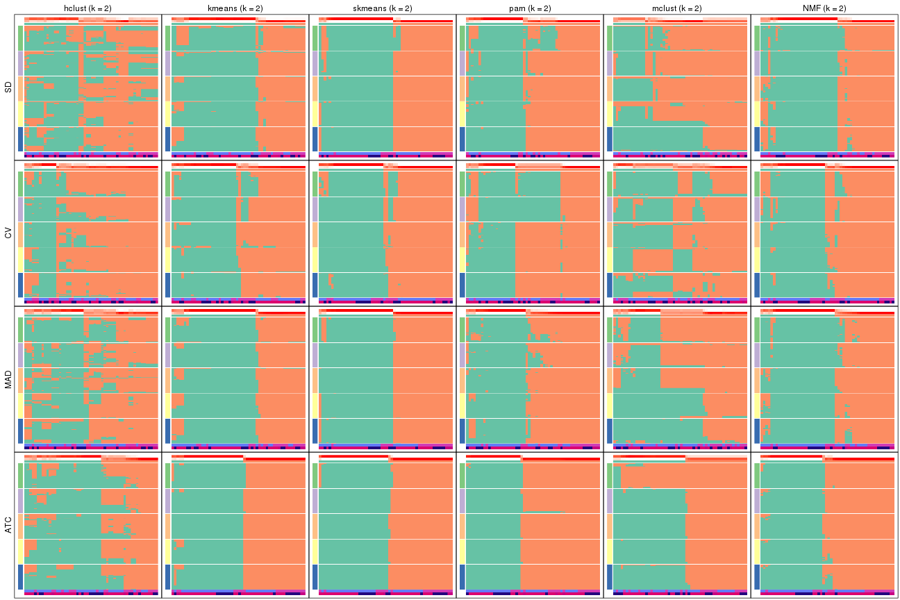
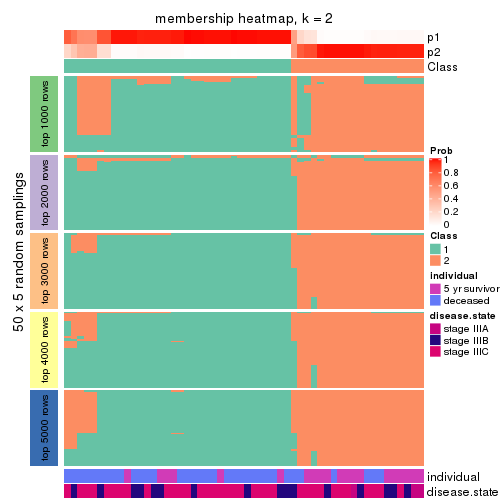
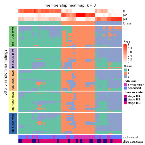
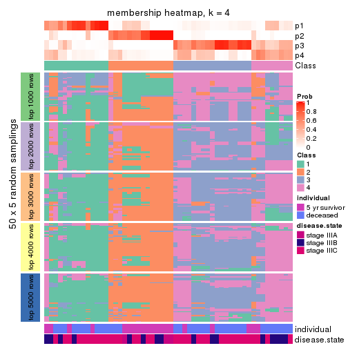
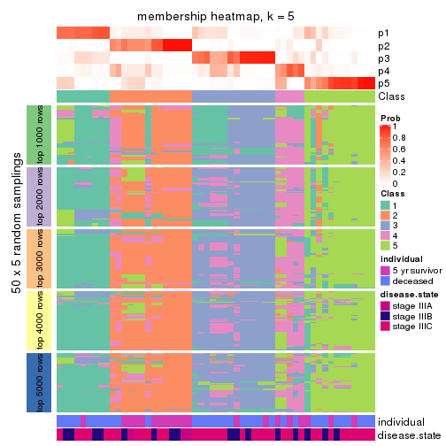
Membership heatmaps for all methods. (What is a membership heatmap?)
collect_plots(res_list, k = 2, fun = membership_heatmap, mc.cores = 4)
collect_plots(res_list, k = 3, fun = membership_heatmap, mc.cores = 4)
collect_plots(res_list, k = 4, fun = membership_heatmap, mc.cores = 4)
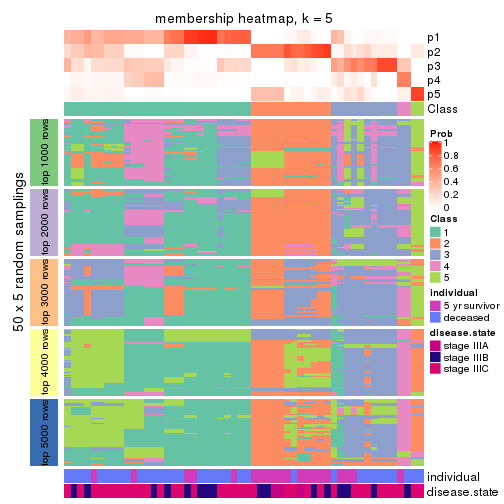
collect_plots(res_list, k = 5, fun = membership_heatmap, mc.cores = 4)
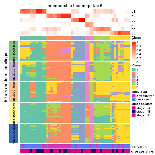
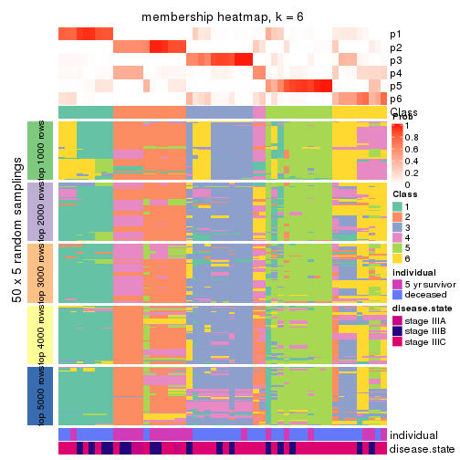
collect_plots(res_list, k = 6, fun = membership_heatmap, mc.cores = 4)
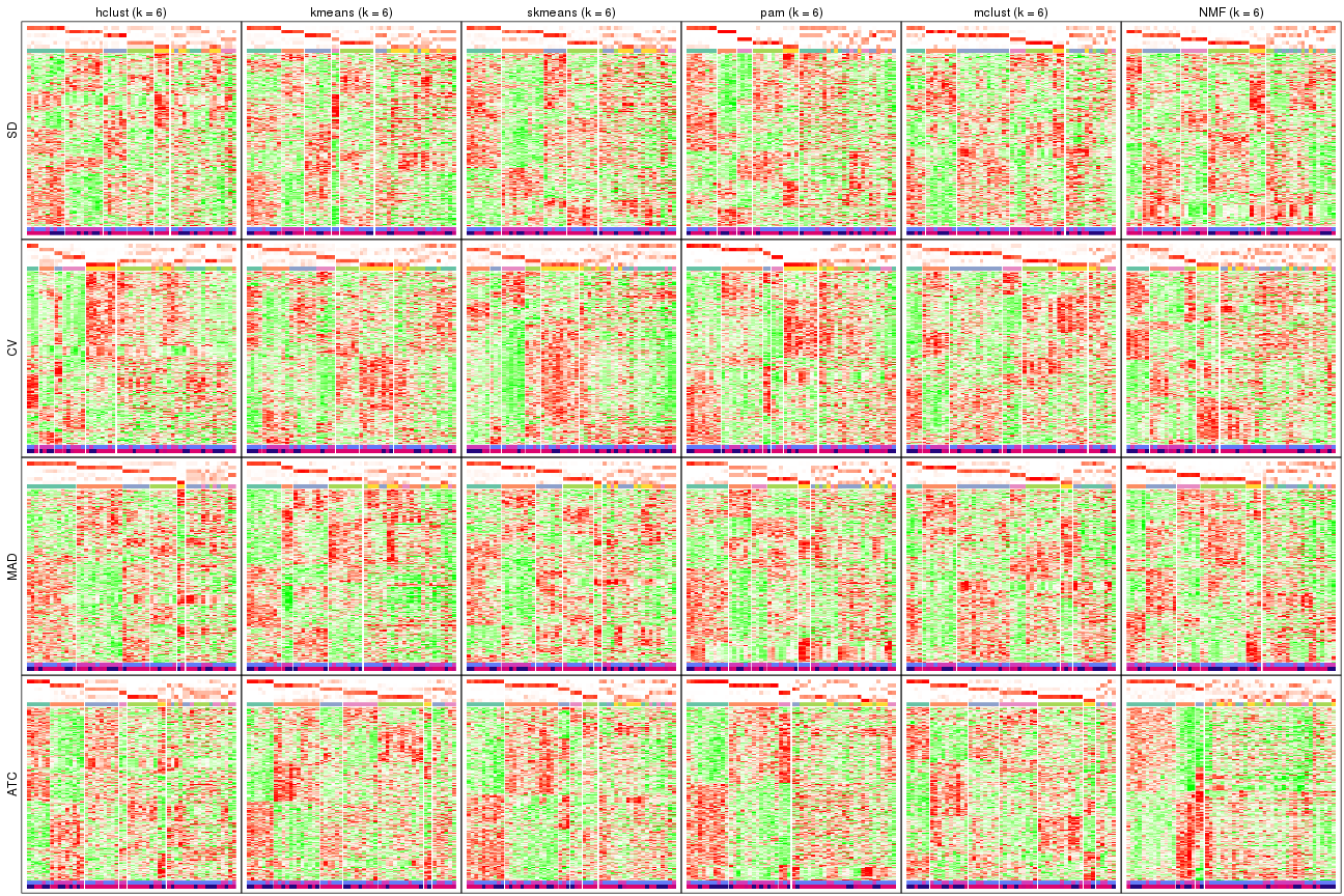
Signature heatmaps for all methods. (What is a signature heatmap?)
Note in following heatmaps, rows are scaled.
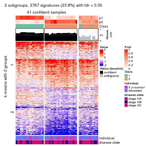
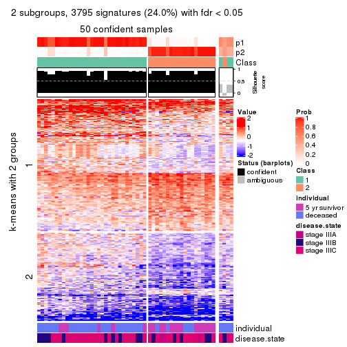
collect_plots(res_list, k = 2, fun = get_signatures, mc.cores = 4)
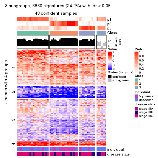
collect_plots(res_list, k = 3, fun = get_signatures, mc.cores = 4)
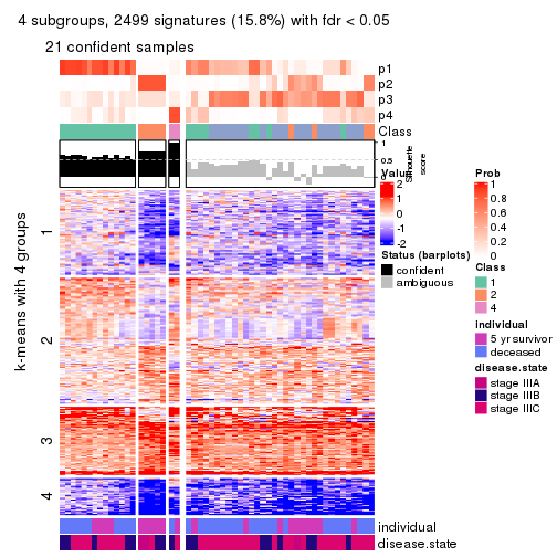
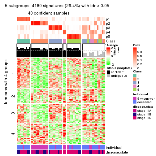
collect_plots(res_list, k = 4, fun = get_signatures, mc.cores = 4)
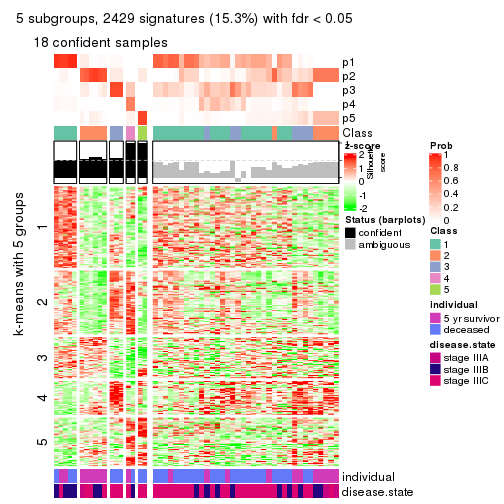
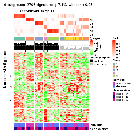
collect_plots(res_list, k = 5, fun = get_signatures, mc.cores = 4)
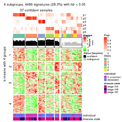
collect_plots(res_list, k = 6, fun = get_signatures, mc.cores = 4)
The statistics used for measuring the stability of consensus partitioning. (How are they defined?)
get_stats(res_list, k = 2)
#>             k  1-PAC mean_silhouette concordance area_increased  Rand Jaccard
#> SD:NMF      2 0.6463           0.842       0.935          0.500 0.502   0.502
#> CV:NMF      2 0.6180           0.847       0.934          0.506 0.491   0.491
#> MAD:NMF     2 0.6769           0.856       0.939          0.497 0.497   0.497
#> ATC:NMF     2 0.8510           0.937       0.973          0.507 0.493   0.493
#> SD:skmeans  2 0.8510           0.923       0.968          0.506 0.497   0.497
#> CV:skmeans  2 0.7522           0.878       0.948          0.509 0.491   0.491
#> MAD:skmeans 2 1.0000           0.960       0.983          0.506 0.497   0.497
#> ATC:skmeans 2 1.0000           0.958       0.984          0.508 0.491   0.491
#> SD:mclust   2 0.3624           0.682       0.815          0.408 0.628   0.628
#> CV:mclust   2 0.2525           0.624       0.787          0.457 0.497   0.497
#> MAD:mclust  2 0.4055           0.555       0.790          0.415 0.535   0.535
#> ATC:mclust  2 0.4902           0.955       0.896          0.429 0.493   0.493
#> SD:kmeans   2 0.7137           0.845       0.925          0.481 0.525   0.525
#> CV:kmeans   2 0.6557           0.854       0.929          0.504 0.491   0.491
#> MAD:kmeans  2 0.8839           0.867       0.948          0.484 0.525   0.525
#> ATC:kmeans  2 0.8871           0.962       0.982          0.507 0.493   0.493
#> SD:pam      2 0.5475           0.853       0.928          0.498 0.502   0.502
#> CV:pam      2 0.4510           0.685       0.823          0.474 0.525   0.525
#> MAD:pam     2 0.7137           0.862       0.938          0.502 0.497   0.497
#> ATC:pam     2 1.0000           0.974       0.986          0.493 0.508   0.508
#> SD:hclust   2 0.0941           0.588       0.751          0.454 0.508   0.508
#> CV:hclust   2 0.4149           0.739       0.875          0.386 0.628   0.628
#> MAD:hclust  2 0.1875           0.562       0.797          0.474 0.497   0.497
#> ATC:hclust  2 0.2886           0.681       0.846          0.448 0.502   0.502
get_stats(res_list, k = 3)
#>             k 1-PAC mean_silhouette concordance area_increased  Rand Jaccard
#> SD:NMF      3 0.437           0.554       0.796          0.315 0.750   0.545
#> CV:NMF      3 0.505           0.736       0.838          0.305 0.688   0.447
#> MAD:NMF     3 0.504           0.660       0.836          0.317 0.790   0.605
#> ATC:NMF     3 0.794           0.807       0.920          0.321 0.753   0.537
#> SD:skmeans  3 0.535           0.792       0.878          0.328 0.743   0.526
#> CV:skmeans  3 0.461           0.591       0.804          0.309 0.716   0.484
#> MAD:skmeans 3 0.675           0.837       0.909          0.324 0.743   0.526
#> ATC:skmeans 3 0.640           0.675       0.819          0.290 0.805   0.623
#> SD:mclust   3 0.291           0.580       0.773          0.416 0.616   0.451
#> CV:mclust   3 0.304           0.425       0.693          0.331 0.491   0.267
#> MAD:mclust  3 0.362           0.574       0.789          0.454 0.644   0.434
#> ATC:mclust  3 0.327           0.474       0.722          0.373 0.869   0.737
#> SD:kmeans   3 0.411           0.644       0.770          0.354 0.774   0.582
#> CV:kmeans   3 0.389           0.510       0.715          0.300 0.782   0.585
#> MAD:kmeans  3 0.449           0.623       0.791          0.350 0.802   0.635
#> ATC:kmeans  3 0.427           0.505       0.744          0.305 0.717   0.485
#> SD:pam      3 0.580           0.781       0.870          0.315 0.704   0.477
#> CV:pam      3 0.490           0.676       0.827          0.360 0.765   0.576
#> MAD:pam     3 0.492           0.706       0.814          0.298 0.728   0.507
#> ATC:pam     3 0.545           0.677       0.824          0.329 0.804   0.625
#> SD:hclust   3 0.154           0.440       0.667          0.323 0.825   0.665
#> CV:hclust   3 0.252           0.520       0.671          0.530 0.647   0.471
#> MAD:hclust  3 0.230           0.369       0.672          0.294 0.795   0.624
#> ATC:hclust  3 0.297           0.517       0.715          0.383 0.737   0.526
get_stats(res_list, k = 4)
#>             k 1-PAC mean_silhouette concordance area_increased  Rand Jaccard
#> SD:NMF      4 0.600           0.694       0.840         0.1199 0.777   0.463
#> CV:NMF      4 0.387           0.384       0.667         0.1250 0.886   0.678
#> MAD:NMF     4 0.629           0.674       0.845         0.1090 0.794   0.505
#> ATC:NMF     4 0.619           0.670       0.820         0.1175 0.814   0.510
#> SD:skmeans  4 0.598           0.622       0.801         0.1285 0.808   0.496
#> CV:skmeans  4 0.457           0.435       0.697         0.1236 0.772   0.427
#> MAD:skmeans 4 0.644           0.629       0.804         0.1309 0.805   0.490
#> ATC:skmeans 4 0.694           0.715       0.870         0.1339 0.826   0.551
#> SD:mclust   4 0.482           0.467       0.761         0.2279 0.748   0.445
#> CV:mclust   4 0.378           0.430       0.696         0.1508 0.811   0.562
#> MAD:mclust  4 0.525           0.469       0.730         0.1935 0.922   0.805
#> ATC:mclust  4 0.432           0.531       0.690         0.2137 0.806   0.534
#> SD:kmeans   4 0.526           0.469       0.664         0.1390 0.837   0.561
#> CV:kmeans   4 0.403           0.482       0.676         0.1310 0.787   0.464
#> MAD:kmeans  4 0.576           0.557       0.716         0.1407 0.812   0.521
#> ATC:kmeans  4 0.586           0.726       0.824         0.1309 0.816   0.507
#> SD:pam      4 0.613           0.651       0.806         0.0931 0.856   0.627
#> CV:pam      4 0.536           0.591       0.792         0.1392 0.827   0.551
#> MAD:pam     4 0.528           0.621       0.761         0.1019 0.869   0.651
#> ATC:pam     4 0.591           0.361       0.730         0.1031 0.876   0.687
#> SD:hclust   4 0.345           0.430       0.650         0.1423 0.920   0.795
#> CV:hclust   4 0.333           0.487       0.692         0.1463 0.763   0.519
#> MAD:hclust  4 0.304           0.352       0.583         0.1091 0.649   0.329
#> ATC:hclust  4 0.396           0.317       0.675         0.1318 0.956   0.877
get_stats(res_list, k = 5)
#>             k 1-PAC mean_silhouette concordance area_increased  Rand Jaccard
#> SD:NMF      5 0.573           0.430       0.708         0.0701 0.908   0.685
#> CV:NMF      5 0.519           0.480       0.718         0.0703 0.832   0.471
#> MAD:NMF     5 0.563           0.450       0.712         0.0777 0.858   0.561
#> ATC:NMF     5 0.549           0.528       0.734         0.0486 0.808   0.412
#> SD:skmeans  5 0.667           0.629       0.793         0.0646 0.872   0.539
#> CV:skmeans  5 0.507           0.483       0.703         0.0664 0.887   0.589
#> MAD:skmeans 5 0.696           0.648       0.798         0.0651 0.899   0.620
#> ATC:skmeans 5 0.675           0.632       0.803         0.0562 0.962   0.851
#> SD:mclust   5 0.628           0.591       0.763         0.0733 0.879   0.622
#> CV:mclust   5 0.480           0.439       0.667         0.0910 0.831   0.486
#> MAD:mclust  5 0.620           0.621       0.799         0.0633 0.843   0.586
#> ATC:mclust  5 0.642           0.736       0.809         0.0822 0.839   0.496
#> SD:kmeans   5 0.636           0.576       0.758         0.0718 0.925   0.714
#> CV:kmeans   5 0.507           0.476       0.631         0.0699 0.905   0.641
#> MAD:kmeans  5 0.642           0.629       0.768         0.0675 0.946   0.782
#> ATC:kmeans  5 0.638           0.595       0.761         0.0627 0.941   0.763
#> SD:pam      5 0.620           0.470       0.736         0.0952 0.871   0.592
#> CV:pam      5 0.592           0.459       0.735         0.0526 0.863   0.545
#> MAD:pam     5 0.616           0.430       0.717         0.0969 0.860   0.550
#> ATC:pam     5 0.693           0.634       0.803         0.0596 0.816   0.492
#> SD:hclust   5 0.426           0.431       0.614         0.0753 0.714   0.406
#> CV:hclust   5 0.464           0.429       0.716         0.1055 0.795   0.506
#> MAD:hclust  5 0.472           0.468       0.649         0.0871 0.860   0.620
#> ATC:hclust  5 0.458           0.396       0.695         0.0614 0.846   0.588
get_stats(res_list, k = 6)
#>             k 1-PAC mean_silhouette concordance area_increased  Rand Jaccard
#> SD:NMF      6 0.661           0.539       0.747         0.0506 0.778   0.303
#> CV:NMF      6 0.546           0.414       0.640         0.0400 0.884   0.513
#> MAD:NMF     6 0.668           0.564       0.752         0.0521 0.785   0.306
#> ATC:NMF     6 0.569           0.429       0.671         0.0432 0.865   0.506
#> SD:skmeans  6 0.696           0.502       0.720         0.0400 0.966   0.828
#> CV:skmeans  6 0.571           0.444       0.673         0.0404 0.919   0.633
#> MAD:skmeans 6 0.693           0.535       0.733         0.0385 0.976   0.879
#> ATC:skmeans 6 0.689           0.556       0.761         0.0382 0.947   0.778
#> SD:mclust   6 0.739           0.612       0.794         0.0546 0.946   0.792
#> CV:mclust   6 0.658           0.660       0.801         0.0615 0.919   0.643
#> MAD:mclust  6 0.692           0.657       0.765         0.0513 0.936   0.747
#> ATC:mclust  6 0.725           0.754       0.827         0.0554 0.928   0.688
#> SD:kmeans   6 0.704           0.507       0.685         0.0422 0.921   0.655
#> CV:kmeans   6 0.591           0.539       0.663         0.0422 0.899   0.558
#> MAD:kmeans  6 0.731           0.564       0.715         0.0418 0.943   0.736
#> ATC:kmeans  6 0.672           0.682       0.743         0.0373 0.941   0.732
#> SD:pam      6 0.702           0.482       0.737         0.0593 0.880   0.529
#> CV:pam      6 0.663           0.516       0.791         0.0339 0.838   0.437
#> MAD:pam     6 0.687           0.504       0.736         0.0520 0.886   0.518
#> ATC:pam     6 0.729           0.544       0.803         0.0370 0.906   0.626
#> SD:hclust   6 0.488           0.568       0.688         0.0606 0.801   0.441
#> CV:hclust   6 0.511           0.386       0.673         0.0531 0.947   0.781
#> MAD:hclust  6 0.555           0.569       0.650         0.0641 0.854   0.537
#> ATC:hclust  6 0.581           0.523       0.690         0.0704 0.865   0.542
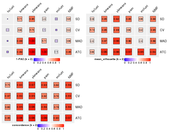
Following heatmap plots the partition for each combination of methods and the lightness correspond to the silhouette scores for samples in each method. On top the consensus subgroup is inferred from all methods by taking the mean silhouette scores as weight.
collect_stats(res_list, k = 2)
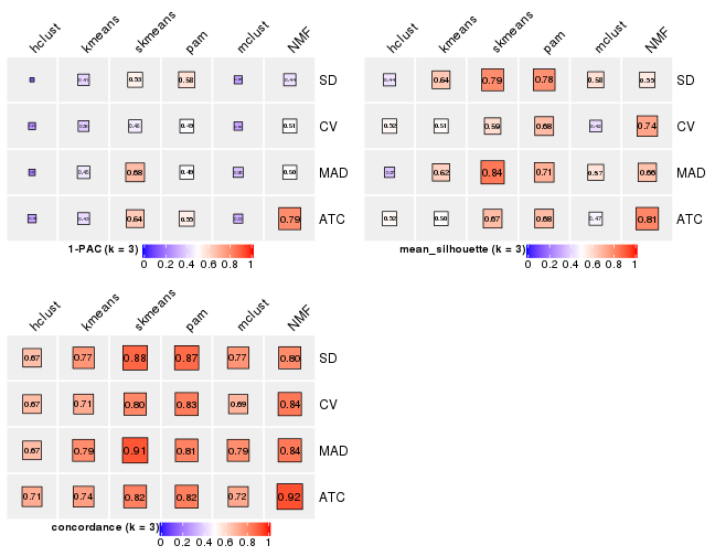
collect_stats(res_list, k = 3)
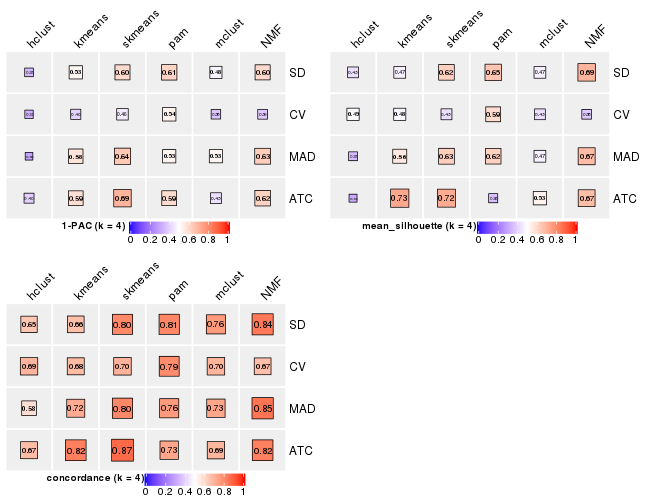
collect_stats(res_list, k = 4)
collect_stats(res_list, k = 5)
collect_stats(res_list, k = 6)
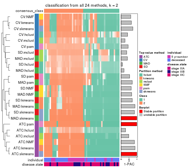
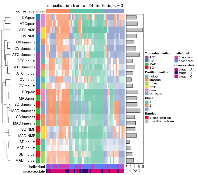
Collect partitions from all methods:
collect_classes(res_list, k = 2)
collect_classes(res_list, k = 3)
collect_classes(res_list, k = 4)
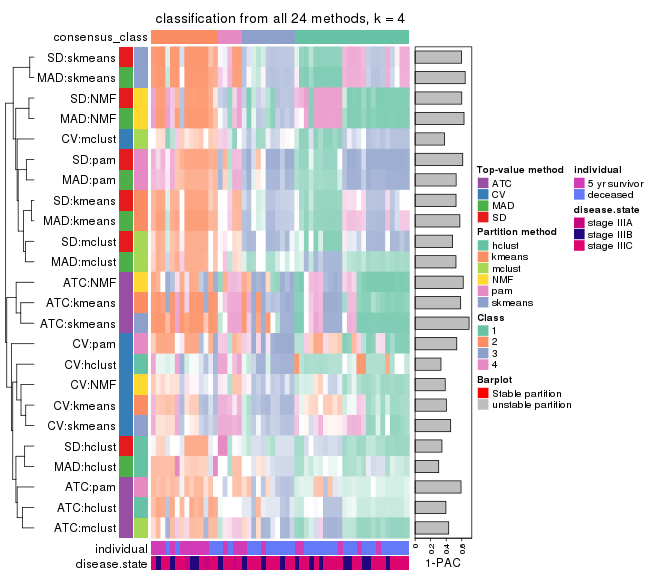
collect_classes(res_list, k = 5)
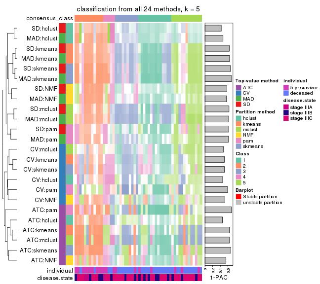
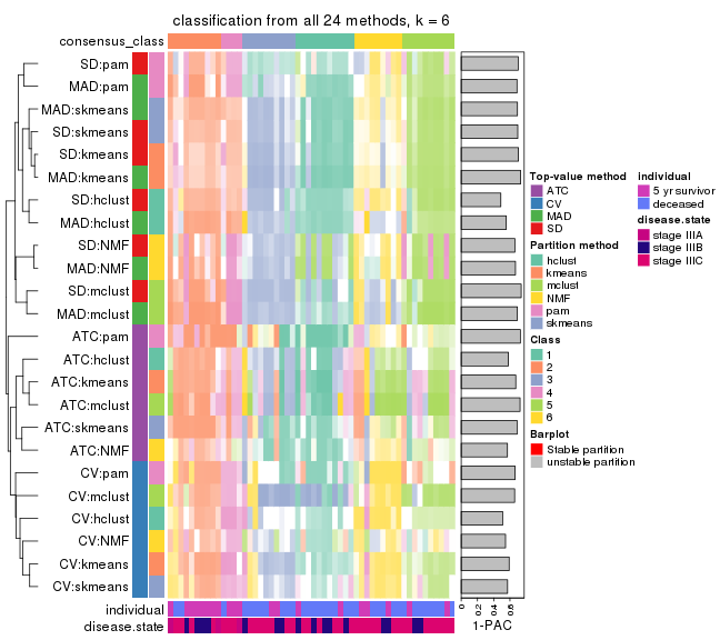
collect_classes(res_list, k = 6)
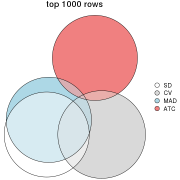
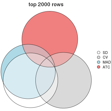
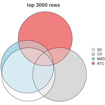
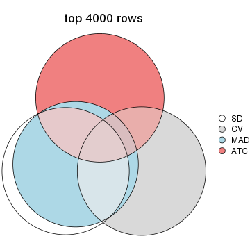
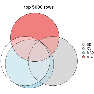
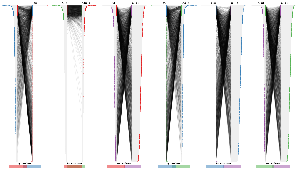
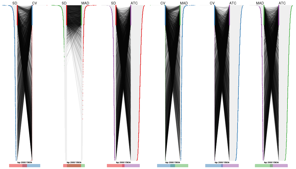
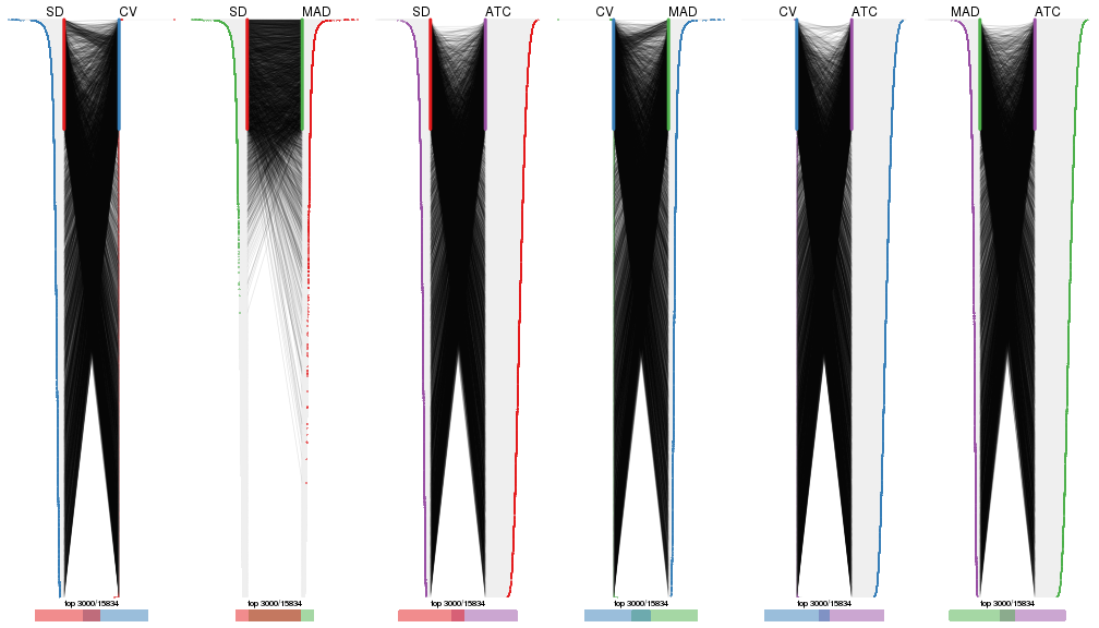
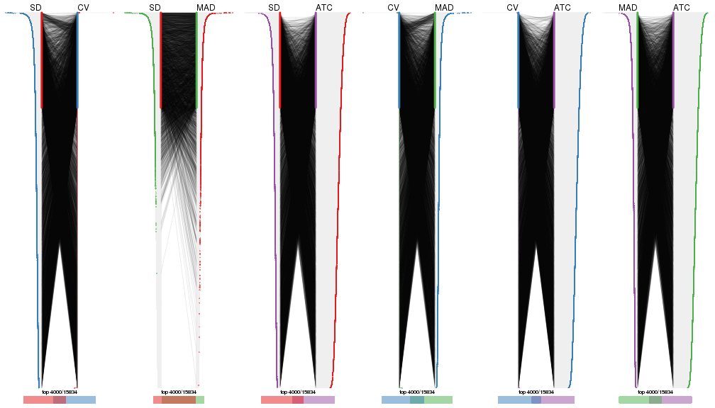
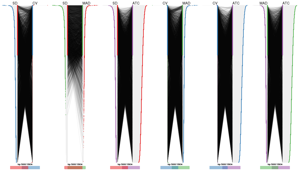
Overlap of top rows from different top-row methods:
top_rows_overlap(res_list, top_n = 1000, method = "euler")
top_rows_overlap(res_list, top_n = 2000, method = "euler")
top_rows_overlap(res_list, top_n = 3000, method = "euler")
top_rows_overlap(res_list, top_n = 4000, method = "euler")
top_rows_overlap(res_list, top_n = 5000, method = "euler")
Also visualize the correspondance of rankings between different top-row methods:
top_rows_overlap(res_list, top_n = 1000, method = "correspondance")
top_rows_overlap(res_list, top_n = 2000, method = "correspondance")
top_rows_overlap(res_list, top_n = 3000, method = "correspondance")
top_rows_overlap(res_list, top_n = 4000, method = "correspondance")
top_rows_overlap(res_list, top_n = 5000, method = "correspondance")
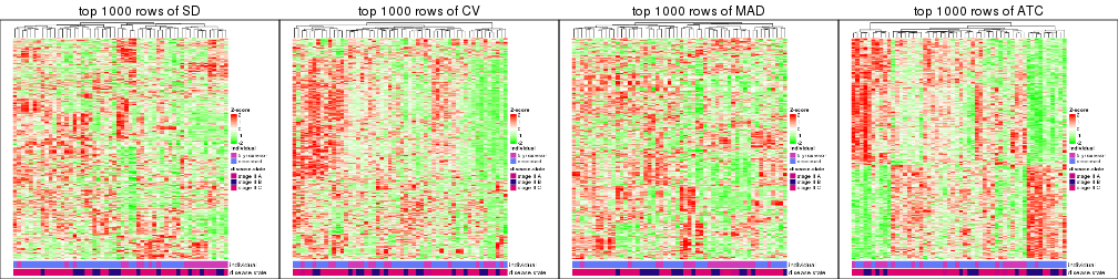
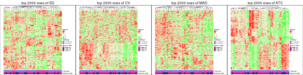
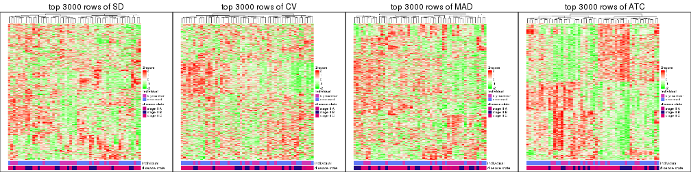
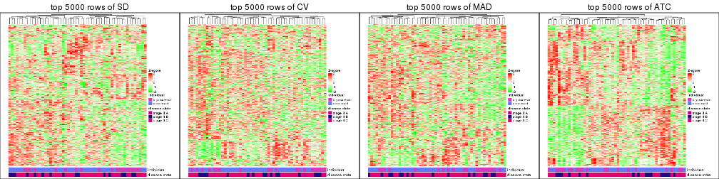
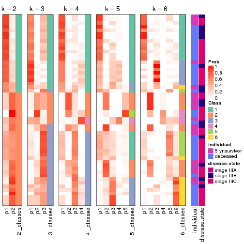
Heatmaps of the top rows:
top_rows_heatmap(res_list, top_n = 1000)
top_rows_heatmap(res_list, top_n = 2000)
top_rows_heatmap(res_list, top_n = 3000)
top_rows_heatmap(res_list, top_n = 4000)
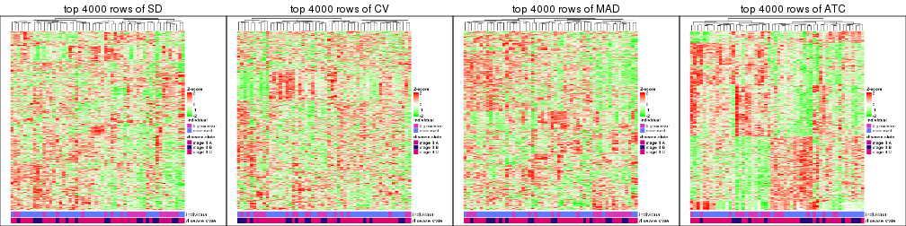
top_rows_heatmap(res_list, top_n = 5000)
Test correlation between subgroups and known annotations. If the known annotation is numeric, one-way ANOVA test is applied, and if the known annotation is discrete, chi-squared contingency table test is applied.
test_to_known_factors(res_list, k = 2)
#>              n individual(p) disease.state(p) k
#> SD:NMF      50       0.00539           0.1356 2
#> CV:NMF      50       0.76828           0.8290 2
#> MAD:NMF     50       0.00627           0.1258 2
#> ATC:NMF     53       0.02554           0.7831 2
#> SD:skmeans  52       0.01464           0.1555 2
#> CV:skmeans  51       0.69173           0.8777 2
#> MAD:skmeans 53       0.01142           0.1443 2
#> ATC:skmeans 53       0.08177           0.7831 2
#> SD:mclust   47       0.06712           0.0848 2
#> CV:mclust   44       0.74619           0.7919 2
#> MAD:mclust  32       0.00372           0.0594 2
#> ATC:mclust  54       0.06702           0.7606 2
#> SD:kmeans   50       0.00045           0.0738 2
#> CV:kmeans   50       0.83900           0.7591 2
#> MAD:kmeans  49       0.00061           0.0799 2
#> ATC:kmeans  54       0.06702           0.7606 2
#> SD:pam      51       0.01163           0.2566 2
#> CV:pam      49       0.03282           0.2943 2
#> MAD:pam     51       0.01788           0.2049 2
#> ATC:pam     53       0.02878           0.1564 2
#> SD:hclust   41       0.03176           0.2472 2
#> CV:hclust   47       0.36959           0.5811 2
#> MAD:hclust  36       0.00278           0.1558 2
#> ATC:hclust  45       0.07400           0.6119 2
test_to_known_factors(res_list, k = 3)
#>              n individual(p) disease.state(p) k
#> SD:NMF      39      0.019984           0.4673 3
#> CV:NMF      49      0.002502           0.1214 3
#> MAD:NMF     44      0.029971           0.4884 3
#> ATC:NMF     48      0.003971           0.4398 3
#> SD:skmeans  52      0.001317           0.1210 3
#> CV:skmeans  39      0.011556           0.5004 3
#> MAD:skmeans 53      0.000999           0.1418 3
#> ATC:skmeans 43      0.332813           0.5971 3
#> SD:mclust   37      0.003023           0.0677 3
#> CV:mclust   29      0.060946           0.0190 3
#> MAD:mclust  41      0.000107           0.0230 3
#> ATC:mclust  36      0.014996           0.1973 3
#> SD:kmeans   48      0.003453           0.1860 3
#> CV:kmeans   38      0.140888           0.3192 3
#> MAD:kmeans  46      0.001024           0.1923 3
#> ATC:kmeans  28      0.009580           1.0000 3
#> SD:pam      48      0.002288           0.1925 3
#> CV:pam      44      0.033068           0.3257 3
#> MAD:pam     48      0.000416           0.1884 3
#> ATC:pam     44      0.011960           0.2406 3
#> SD:hclust   21      0.966852           0.9064 3
#> CV:hclust   34      0.442078           0.6559 3
#> MAD:hclust  19            NA               NA 3
#> ATC:hclust  36      0.015871           0.3537 3
test_to_known_factors(res_list, k = 4)
#>              n individual(p) disease.state(p) k
#> SD:NMF      46      0.010215           0.1545 4
#> CV:NMF      20      0.023139           0.0427 4
#> MAD:NMF     47      0.012790           0.3183 4
#> ATC:NMF     47      0.055778           0.5247 4
#> SD:skmeans  42      0.001872           0.1812 4
#> CV:skmeans  27      0.066611           0.6404 4
#> MAD:skmeans 42      0.001945           0.2124 4
#> ATC:skmeans 45      0.077136           0.8199 4
#> SD:mclust   31      0.001662           0.0361 4
#> CV:mclust   23      0.367054           0.5440 4
#> MAD:mclust  32      0.002643           0.1877 4
#> ATC:mclust  31      0.128063           0.3407 4
#> SD:kmeans   30      0.001112           0.1296 4
#> CV:kmeans   28      0.162290           0.8140 4
#> MAD:kmeans  38      0.002022           0.1480 4
#> ATC:kmeans  49      0.017027           0.5443 4
#> SD:pam      47      0.000437           0.3489 4
#> CV:pam      31      0.007443           0.3569 4
#> MAD:pam     45      0.000262           0.3261 4
#> ATC:pam     23      0.158259           0.6193 4
#> SD:hclust   21      0.023042           0.0960 4
#> CV:hclust   32      0.174801           0.3076 4
#> MAD:hclust  17      0.023067           0.3279 4
#> ATC:hclust  19      0.033121           0.5230 4
test_to_known_factors(res_list, k = 5)
#>              n individual(p) disease.state(p) k
#> SD:NMF      22      5.06e-02           0.1457 5
#> CV:NMF      31      7.49e-02           0.1093 5
#> MAD:NMF     29      3.04e-02           0.3140 5
#> ATC:NMF     37      3.21e-01           0.5261 5
#> SD:skmeans  38      2.94e-04           0.1559 5
#> CV:skmeans  34      9.87e-03           0.2279 5
#> MAD:skmeans 39      6.68e-04           0.1256 5
#> ATC:skmeans 41      5.68e-02           0.5886 5
#> SD:mclust   41      3.36e-04           0.0457 5
#> CV:mclust   25      5.74e-01           0.4232 5
#> MAD:mclust  41      1.49e-03           0.1297 5
#> ATC:mclust  47      2.88e-02           0.0557 5
#> SD:kmeans   40      2.68e-05           0.1494 5
#> CV:kmeans   34      3.70e-03           0.0993 5
#> MAD:kmeans  41      1.21e-04           0.2202 5
#> ATC:kmeans  39      1.95e-02           0.4290 5
#> SD:pam      31      5.19e-04           0.1493 5
#> CV:pam      29      5.47e-03           0.3194 5
#> MAD:pam     30      2.34e-03           0.2136 5
#> ATC:pam     38      1.59e-02           0.4857 5
#> SD:hclust   18      2.44e-02           0.3266 5
#> CV:hclust   23      1.19e-01           0.2918 5
#> MAD:hclust  24      7.38e-03           0.3847 5
#> ATC:hclust  23      3.29e-02           0.0412 5
test_to_known_factors(res_list, k = 6)
#>              n individual(p) disease.state(p) k
#> SD:NMF      36      0.002007          0.05338 6
#> CV:NMF      25      0.068341          0.53332 6
#> MAD:NMF     35      0.009868          0.04785 6
#> ATC:NMF     21      0.127044          0.39699 6
#> SD:skmeans  34      0.000109          0.09577 6
#> CV:skmeans  29      0.022306          0.16034 6
#> MAD:skmeans 35      0.002263          0.14685 6
#> ATC:skmeans 34      0.366077          0.10773 6
#> SD:mclust   41      0.002198          0.08998 6
#> CV:mclust   47      0.022474          0.18021 6
#> MAD:mclust  43      0.001236          0.28307 6
#> ATC:mclust  49      0.138570          0.03453 6
#> SD:kmeans   33      0.001639          0.55186 6
#> CV:kmeans   38      0.041477          0.22965 6
#> MAD:kmeans  30      0.009901          0.39163 6
#> ATC:kmeans  48      0.035493          0.27041 6
#> SD:pam      30      0.001195          0.27936 6
#> CV:pam      34      0.058640          0.65824 6
#> MAD:pam     32      0.001145          0.20199 6
#> ATC:pam     27      0.014039          0.51692 6
#> SD:hclust   37      0.000985          0.06870 6
#> CV:hclust   23      0.061766          0.33643 6
#> MAD:hclust  41      0.000945          0.19514 6
#> ATC:hclust  36      0.031076          0.00154 6
The object with results only for a single top-value method and a single partition method can be extracted as:
res = res_list["SD", "hclust"]
# you can also extract it by
# res = res_list["SD:hclust"]
A summary of res and all the functions that can be applied to it:
res
#> A 'ConsensusPartition' object with k = 2, 3, 4, 5, 6.
#>   On a matrix with 15834 rows and 54 columns.
#>   Top rows (1000, 2000, 3000, 4000, 5000) are extracted by 'SD' method.
#>   Subgroups are detected by 'hclust' method.
#>   Performed in total 1250 partitions by row resampling.
#>   Best k for subgroups seems to be 2.
#>
#> Following methods can be applied to this 'ConsensusPartition' object:
#>  [1] "cola_report"             "collect_classes"         "collect_plots"
#>  [4] "collect_stats"           "colnames"                "compare_signatures"
#>  [7] "consensus_heatmap"       "dimension_reduction"     "functional_enrichment"
#> [10] "get_anno_col"            "get_anno"                "get_classes"
#> [13] "get_consensus"           "get_matrix"              "get_membership"
#> [16] "get_param"               "get_signatures"          "get_stats"
#> [19] "is_best_k"               "is_stable_k"             "membership_heatmap"
#> [22] "ncol"                    "nrow"                    "plot_ecdf"
#> [25] "rownames"                "select_partition_number" "show"
#> [28] "suggest_best_k"          "test_to_known_factors"
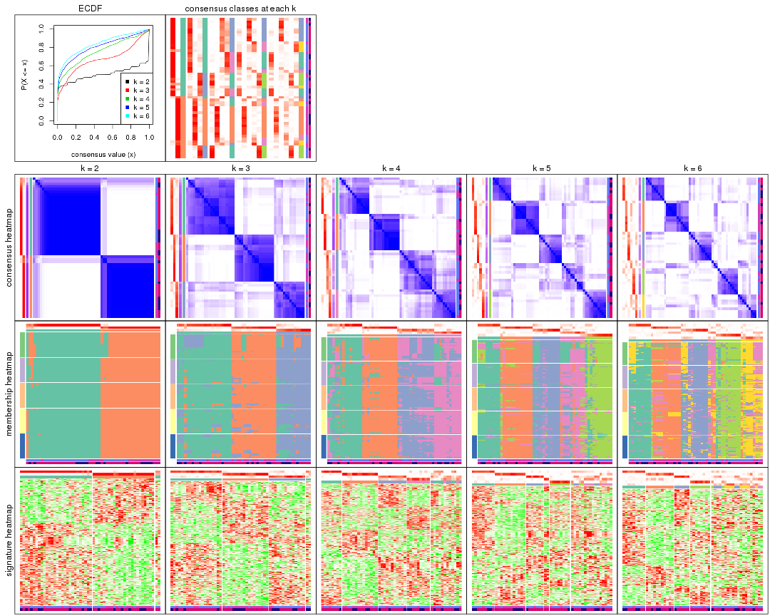
collect_plots() function collects all the plots made from res for all k (number of partitions)
into one single page to provide an easy and fast comparison between different k.
collect_plots(res)
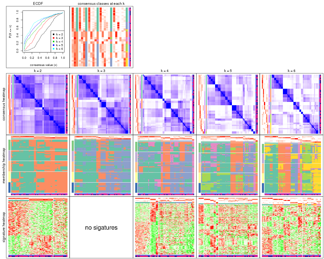
The plots are:
k and the heatmap of
predicted classes for each k.k.k.k.All the plots in panels can be made by individual functions and they are plotted later in this section.
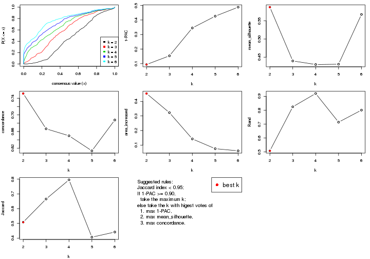
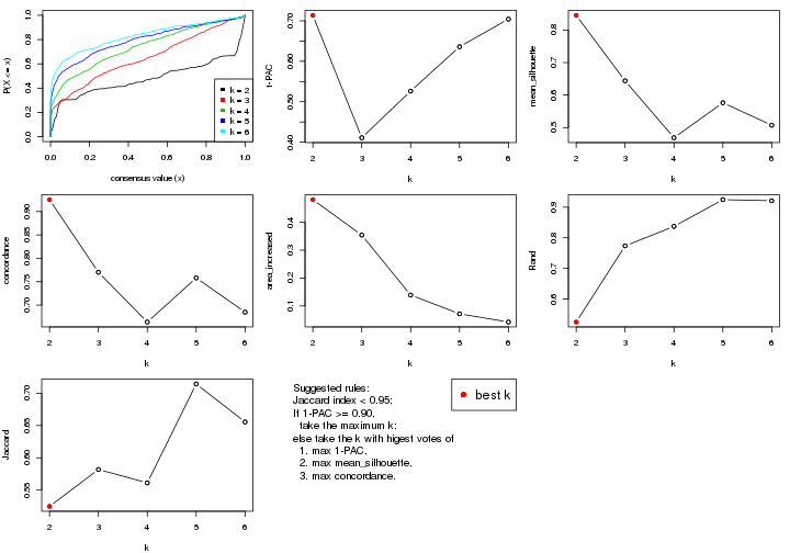
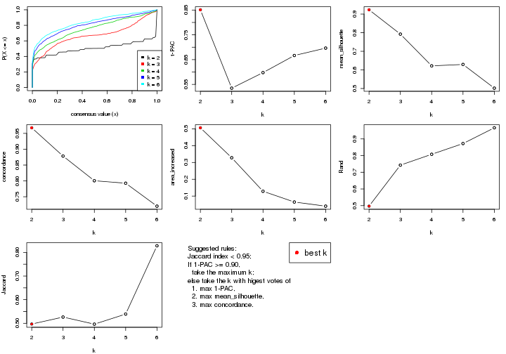
select_partition_number() produces several plots showing different
statistics for choosing “optimized” k. There are following statistics:
k;k, the area increased is defined as \(A_k - A_{k-1}\).The detailed explanations of these statistics can be found in the cola vignette.
Generally speaking, lower PAC score, higher mean silhouette score or higher
concordance corresponds to better partition. Rand index and Jaccard index
measure how similar the current partition is compared to partition with k-1.
If they are too similar, we won't accept k is better than k-1.
select_partition_number(res)
The numeric values for all these statistics can be obtained by get_stats().
get_stats(res)
#>   k  1-PAC mean_silhouette concordance area_increased  Rand Jaccard
#> 2 2 0.0941           0.588       0.751         0.4541 0.508   0.508
#> 3 3 0.1537           0.440       0.667         0.3227 0.825   0.665
#> 4 4 0.3451           0.430       0.650         0.1423 0.920   0.795
#> 5 5 0.4261           0.431       0.614         0.0753 0.714   0.406
#> 6 6 0.4879           0.568       0.688         0.0606 0.801   0.441
suggest_best_k() suggests the best \(k\) based on these statistics. The rules are as follows:
suggest_best_k(res)
#> [1] 2
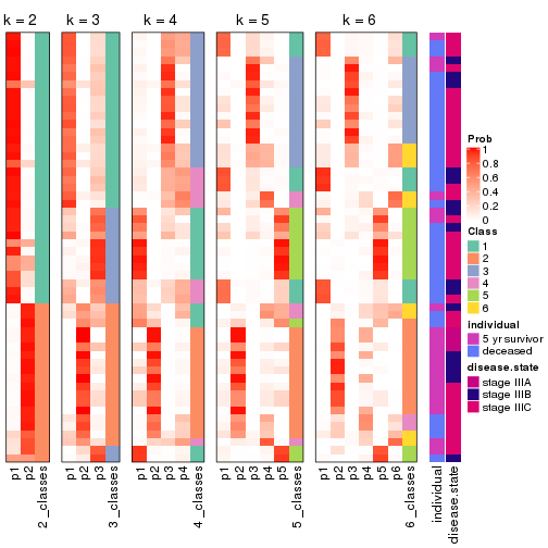
Following shows the table of the partitions (You need to click the show/hide
code output link to see it). The membership matrix (columns with name p*)
is inferred by
clue::cl_consensus()
function with the SE method. Basically the value in the membership matrix
represents the probability to belong to a certain group. The finall class
label for an item is determined with the group with highest probability it
belongs to.
In get_classes() function, the entropy is calculated from the membership
matrix and the silhouette score is calculated from the consensus matrix.
cbind(get_classes(res, k = 2), get_membership(res, k = 2))
#>           class entropy silhouette    p1    p2
#> GSM311939     2  0.7815      0.678 0.232 0.768
#> GSM311963     2  0.7815      0.678 0.232 0.768
#> GSM311973     2  0.8763      0.645 0.296 0.704
#> GSM311940     2  0.7815      0.678 0.232 0.768
#> GSM311953     2  0.8267      0.667 0.260 0.740
#> GSM311974     2  0.8016      0.680 0.244 0.756
#> GSM311975     1  0.9775      0.295 0.588 0.412
#> GSM311977     2  0.7815      0.678 0.232 0.768
#> GSM311982     1  0.4690      0.727 0.900 0.100
#> GSM311990     2  0.5059      0.660 0.112 0.888
#> GSM311943     1  0.7674      0.645 0.776 0.224
#> GSM311944     1  0.4690      0.727 0.900 0.100
#> GSM311946     2  0.8327      0.665 0.264 0.736
#> GSM311956     2  0.7528      0.685 0.216 0.784
#> GSM311967     2  0.3879      0.582 0.076 0.924
#> GSM311968     2  0.9815      0.483 0.420 0.580
#> GSM311972     1  0.4690      0.732 0.900 0.100
#> GSM311980     2  0.8763      0.645 0.296 0.704
#> GSM311981     2  0.9170      0.140 0.332 0.668
#> GSM311988     2  0.7815      0.678 0.232 0.768
#> GSM311957     1  0.9358      0.111 0.648 0.352
#> GSM311960     2  0.9933      0.404 0.452 0.548
#> GSM311971     1  0.3274      0.725 0.940 0.060
#> GSM311976     1  0.6531      0.668 0.832 0.168
#> GSM311978     1  0.2778      0.726 0.952 0.048
#> GSM311979     1  0.3274      0.725 0.940 0.060
#> GSM311983     1  0.7056      0.651 0.808 0.192
#> GSM311986     2  0.9248      0.523 0.340 0.660
#> GSM311991     2  0.9170      0.140 0.332 0.668
#> GSM311938     2  0.7528      0.635 0.216 0.784
#> GSM311941     2  0.9933      0.417 0.452 0.548
#> GSM311942     2  0.9988      0.362 0.480 0.520
#> GSM311945     2  0.9993      0.357 0.484 0.516
#> GSM311947     2  0.1843      0.613 0.028 0.972
#> GSM311948     2  0.7602      0.684 0.220 0.780
#> GSM311949     1  0.6048      0.679 0.852 0.148
#> GSM311950     2  0.0376      0.611 0.004 0.996
#> GSM311951     2  0.9983      0.370 0.476 0.524
#> GSM311952     1  0.7674      0.645 0.776 0.224
#> GSM311954     2  0.7528      0.631 0.216 0.784
#> GSM311955     1  0.9608      0.390 0.616 0.384
#> GSM311958     1  0.5408      0.727 0.876 0.124
#> GSM311959     2  0.7528      0.631 0.216 0.784
#> GSM311961     1  0.7139      0.652 0.804 0.196
#> GSM311962     1  0.4431      0.740 0.908 0.092
#> GSM311964     1  0.6148      0.673 0.848 0.152
#> GSM311965     2  0.9815      0.483 0.420 0.580
#> GSM311966     1  0.4690      0.737 0.900 0.100
#> GSM311969     1  0.7883      0.635 0.764 0.236
#> GSM311970     2  0.0376      0.611 0.004 0.996
#> GSM311984     1  0.7056      0.651 0.808 0.192
#> GSM311985     1  0.5178      0.726 0.884 0.116
#> GSM311987     2  0.7528      0.631 0.216 0.784
#> GSM311989     2  0.9933      0.404 0.452 0.548
cbind(get_classes(res, k = 3), get_membership(res, k = 3))
#>           class entropy silhouette    p1    p2    p3
#> GSM311939     2   0.809    0.44741 0.068 0.516 0.416
#> GSM311963     2   0.809    0.44741 0.068 0.516 0.416
#> GSM311973     3   0.597    0.30784 0.032 0.216 0.752
#> GSM311940     2   0.809    0.44741 0.068 0.516 0.416
#> GSM311953     3   0.751    0.13804 0.068 0.288 0.644
#> GSM311974     3   0.623    0.26782 0.028 0.252 0.720
#> GSM311975     1   0.914    0.26004 0.544 0.208 0.248
#> GSM311977     2   0.809    0.44741 0.068 0.516 0.416
#> GSM311982     1   0.648    0.61755 0.600 0.008 0.392
#> GSM311990     3   0.731    0.33890 0.036 0.384 0.580
#> GSM311943     1   0.414    0.61930 0.860 0.016 0.124
#> GSM311944     1   0.648    0.61755 0.600 0.008 0.392
#> GSM311946     3   0.767    0.09363 0.072 0.300 0.628
#> GSM311956     3   0.435    0.39766 0.000 0.184 0.816
#> GSM311967     3   0.772    0.20729 0.048 0.432 0.520
#> GSM311968     3   0.397    0.53405 0.100 0.024 0.876
#> GSM311972     1   0.637    0.67515 0.668 0.016 0.316
#> GSM311980     3   0.506    0.41178 0.032 0.148 0.820
#> GSM311981     2   0.879   -0.00323 0.428 0.460 0.112
#> GSM311988     2   0.809    0.44741 0.068 0.516 0.416
#> GSM311957     3   0.587    0.13264 0.312 0.004 0.684
#> GSM311960     3   0.517    0.47435 0.116 0.056 0.828
#> GSM311971     1   0.627    0.64546 0.644 0.008 0.348
#> GSM311976     1   0.661    0.55132 0.560 0.008 0.432
#> GSM311978     1   0.610    0.66417 0.672 0.008 0.320
#> GSM311979     1   0.627    0.64546 0.644 0.008 0.348
#> GSM311983     1   0.216    0.55913 0.936 0.064 0.000
#> GSM311986     3   0.963    0.28753 0.364 0.208 0.428
#> GSM311991     2   0.879   -0.00323 0.428 0.460 0.112
#> GSM311938     3   0.977    0.14408 0.232 0.364 0.404
#> GSM311941     3   0.747    0.42133 0.272 0.072 0.656
#> GSM311942     3   0.454    0.46842 0.148 0.016 0.836
#> GSM311945     3   0.480    0.46163 0.156 0.020 0.824
#> GSM311947     3   0.694    0.22426 0.016 0.464 0.520
#> GSM311948     3   0.341    0.45394 0.000 0.124 0.876
#> GSM311949     1   0.660    0.54350 0.564 0.008 0.428
#> GSM311950     2   0.286    0.39286 0.004 0.912 0.084
#> GSM311951     3   0.462    0.47152 0.144 0.020 0.836
#> GSM311952     1   0.414    0.61930 0.860 0.016 0.124
#> GSM311954     3   0.936    0.32674 0.240 0.244 0.516
#> GSM311955     1   0.698    0.49342 0.708 0.072 0.220
#> GSM311958     1   0.630    0.67745 0.712 0.028 0.260
#> GSM311959     3   0.936    0.32674 0.240 0.244 0.516
#> GSM311961     1   0.240    0.56144 0.932 0.064 0.004
#> GSM311962     1   0.614    0.68603 0.684 0.012 0.304
#> GSM311964     1   0.661    0.53629 0.560 0.008 0.432
#> GSM311965     3   0.404    0.53465 0.104 0.024 0.872
#> GSM311966     1   0.628    0.68271 0.680 0.016 0.304
#> GSM311969     1   0.434    0.61571 0.848 0.016 0.136
#> GSM311970     2   0.286    0.39286 0.004 0.912 0.084
#> GSM311984     1   0.216    0.55913 0.936 0.064 0.000
#> GSM311985     1   0.647    0.66636 0.652 0.016 0.332
#> GSM311987     3   0.936    0.32674 0.240 0.244 0.516
#> GSM311989     3   0.517    0.47435 0.116 0.056 0.828
cbind(get_classes(res, k = 4), get_membership(res, k = 4))
#>           class entropy silhouette    p1    p2    p3    p4
#> GSM311939     2   0.379    0.73117 0.016 0.820 0.164 0.000
#> GSM311963     2   0.379    0.73117 0.016 0.820 0.164 0.000
#> GSM311973     3   0.680   -0.12313 0.096 0.448 0.456 0.000
#> GSM311940     2   0.379    0.73117 0.016 0.820 0.164 0.000
#> GSM311953     2   0.554    0.37222 0.020 0.556 0.424 0.000
#> GSM311974     3   0.569   -0.22974 0.024 0.460 0.516 0.000
#> GSM311975     1   0.764    0.23637 0.508 0.016 0.328 0.148
#> GSM311977     2   0.379    0.73117 0.016 0.820 0.164 0.000
#> GSM311982     1   0.350    0.59489 0.832 0.000 0.160 0.008
#> GSM311990     3   0.534    0.41653 0.064 0.008 0.748 0.180
#> GSM311943     1   0.662    0.53622 0.652 0.008 0.152 0.188
#> GSM311944     1   0.350    0.59489 0.832 0.000 0.160 0.008
#> GSM311946     2   0.560    0.40597 0.024 0.568 0.408 0.000
#> GSM311956     3   0.532    0.08852 0.020 0.352 0.628 0.000
#> GSM311967     3   0.636    0.22958 0.044 0.024 0.628 0.304
#> GSM311968     3   0.534    0.44339 0.300 0.032 0.668 0.000
#> GSM311972     1   0.299    0.64692 0.892 0.008 0.016 0.084
#> GSM311980     3   0.670    0.09289 0.096 0.372 0.532 0.000
#> GSM311981     4   0.417    1.00000 0.052 0.012 0.096 0.840
#> GSM311988     2   0.379    0.73117 0.016 0.820 0.164 0.000
#> GSM311957     1   0.736   -0.10337 0.460 0.124 0.408 0.008
#> GSM311960     3   0.511    0.37574 0.328 0.000 0.656 0.016
#> GSM311971     1   0.283    0.62693 0.876 0.000 0.120 0.004
#> GSM311976     1   0.624    0.51314 0.720 0.124 0.124 0.032
#> GSM311978     1   0.240    0.63794 0.904 0.000 0.092 0.004
#> GSM311979     1   0.283    0.62693 0.876 0.000 0.120 0.004
#> GSM311983     1   0.609    0.41729 0.632 0.012 0.044 0.312
#> GSM311986     3   0.683    0.34151 0.252 0.012 0.620 0.116
#> GSM311991     4   0.417    1.00000 0.052 0.012 0.096 0.840
#> GSM311938     3   0.879    0.17445 0.164 0.168 0.520 0.148
#> GSM311941     3   0.652    0.33045 0.384 0.032 0.556 0.028
#> GSM311942     3   0.502    0.36187 0.360 0.000 0.632 0.008
#> GSM311945     3   0.506    0.35542 0.368 0.000 0.624 0.008
#> GSM311947     3   0.491    0.32253 0.012 0.016 0.740 0.232
#> GSM311948     3   0.501    0.24981 0.024 0.276 0.700 0.000
#> GSM311949     1   0.576    0.49880 0.724 0.128 0.144 0.004
#> GSM311950     2   0.650   -0.00936 0.000 0.616 0.116 0.268
#> GSM311951     3   0.501    0.36521 0.356 0.000 0.636 0.008
#> GSM311952     1   0.662    0.53622 0.652 0.008 0.152 0.188
#> GSM311954     3   0.677    0.32953 0.168 0.020 0.660 0.152
#> GSM311955     1   0.764    0.38629 0.536 0.012 0.212 0.240
#> GSM311958     1   0.433    0.62586 0.832 0.012 0.060 0.096
#> GSM311959     3   0.677    0.32953 0.168 0.020 0.660 0.152
#> GSM311961     1   0.616    0.42056 0.628 0.012 0.048 0.312
#> GSM311962     1   0.289    0.65655 0.896 0.004 0.020 0.080
#> GSM311964     1   0.580    0.49462 0.720 0.128 0.148 0.004
#> GSM311965     3   0.537    0.44257 0.304 0.032 0.664 0.000
#> GSM311966     1   0.307    0.65363 0.888 0.004 0.024 0.084
#> GSM311969     1   0.662    0.52937 0.652 0.008 0.152 0.188
#> GSM311970     2   0.650   -0.00936 0.000 0.616 0.116 0.268
#> GSM311984     1   0.609    0.41729 0.632 0.012 0.044 0.312
#> GSM311985     1   0.344    0.64360 0.876 0.008 0.036 0.080
#> GSM311987     3   0.677    0.32953 0.168 0.020 0.660 0.152
#> GSM311989     3   0.511    0.37574 0.328 0.000 0.656 0.016
cbind(get_classes(res, k = 5), get_membership(res, k = 5))
#>           class entropy silhouette    p1    p2    p3    p4    p5
#> GSM311939     2   0.395    0.46377 0.000 0.668 0.000 0.000 0.332
#> GSM311963     2   0.395    0.46377 0.000 0.668 0.000 0.000 0.332
#> GSM311973     2   0.553    0.55198 0.100 0.736 0.092 0.008 0.064
#> GSM311940     2   0.395    0.46377 0.000 0.668 0.000 0.000 0.332
#> GSM311953     2   0.230    0.60790 0.008 0.904 0.008 0.000 0.080
#> GSM311974     2   0.357    0.60328 0.024 0.856 0.064 0.004 0.052
#> GSM311975     3   0.827    0.19576 0.312 0.048 0.416 0.172 0.052
#> GSM311977     2   0.395    0.46377 0.000 0.668 0.000 0.000 0.332
#> GSM311982     1   0.250    0.50937 0.904 0.060 0.012 0.024 0.000
#> GSM311990     3   0.769    0.38563 0.060 0.188 0.548 0.040 0.164
#> GSM311943     1   0.730    0.20138 0.440 0.032 0.268 0.260 0.000
#> GSM311944     1   0.250    0.50937 0.904 0.060 0.012 0.024 0.000
#> GSM311946     2   0.284    0.60322 0.012 0.880 0.020 0.000 0.088
#> GSM311956     2   0.373    0.54417 0.024 0.828 0.128 0.008 0.012
#> GSM311967     3   0.625    0.34289 0.000 0.120 0.664 0.100 0.116
#> GSM311968     1   0.824    0.22256 0.368 0.360 0.180 0.040 0.052
#> GSM311972     1   0.360    0.43141 0.776 0.000 0.212 0.012 0.000
#> GSM311980     2   0.446    0.53208 0.100 0.784 0.104 0.008 0.004
#> GSM311981     4   0.519    1.00000 0.000 0.000 0.280 0.644 0.076
#> GSM311988     2   0.395    0.46377 0.000 0.668 0.000 0.000 0.332
#> GSM311957     1   0.664    0.35867 0.520 0.368 0.044 0.020 0.048
#> GSM311960     1   0.857    0.28992 0.424 0.272 0.168 0.052 0.084
#> GSM311971     1   0.154    0.50693 0.948 0.008 0.008 0.036 0.000
#> GSM311976     1   0.582    0.44328 0.656 0.216 0.108 0.016 0.004
#> GSM311978     1   0.184    0.50463 0.936 0.008 0.016 0.040 0.000
#> GSM311979     1   0.154    0.50693 0.948 0.008 0.008 0.036 0.000
#> GSM311983     1   0.722    0.12826 0.372 0.000 0.256 0.352 0.020
#> GSM311986     3   0.607    0.48114 0.044 0.108 0.676 0.164 0.008
#> GSM311991     4   0.519    1.00000 0.000 0.000 0.280 0.644 0.076
#> GSM311938     3   0.560    0.41820 0.032 0.224 0.672 0.000 0.072
#> GSM311941     1   0.751   -0.00664 0.384 0.188 0.380 0.004 0.044
#> GSM311942     1   0.810    0.30206 0.464 0.248 0.196 0.040 0.052
#> GSM311945     1   0.820    0.30416 0.460 0.240 0.200 0.044 0.056
#> GSM311947     3   0.689    0.37225 0.004 0.168 0.576 0.048 0.204
#> GSM311948     2   0.495    0.45116 0.024 0.752 0.160 0.008 0.056
#> GSM311949     1   0.518    0.45686 0.704 0.220 0.052 0.020 0.004
#> GSM311950     5   0.234    1.00000 0.000 0.112 0.000 0.004 0.884
#> GSM311951     1   0.816    0.30033 0.460 0.248 0.196 0.040 0.056
#> GSM311952     1   0.730    0.20138 0.440 0.032 0.268 0.260 0.000
#> GSM311954     3   0.293    0.56051 0.032 0.104 0.864 0.000 0.000
#> GSM311955     3   0.653   -0.11536 0.380 0.032 0.492 0.096 0.000
#> GSM311958     1   0.413    0.36845 0.696 0.000 0.292 0.012 0.000
#> GSM311959     3   0.293    0.56051 0.032 0.104 0.864 0.000 0.000
#> GSM311961     1   0.722    0.13168 0.376 0.000 0.256 0.348 0.020
#> GSM311962     1   0.377    0.44506 0.780 0.008 0.200 0.012 0.000
#> GSM311964     1   0.509    0.45635 0.708 0.220 0.052 0.016 0.004
#> GSM311965     1   0.824    0.22298 0.372 0.356 0.180 0.040 0.052
#> GSM311966     1   0.384    0.44009 0.772 0.008 0.208 0.012 0.000
#> GSM311969     1   0.728    0.18880 0.436 0.032 0.304 0.228 0.000
#> GSM311970     5   0.234    1.00000 0.000 0.112 0.000 0.004 0.884
#> GSM311984     1   0.722    0.12826 0.372 0.000 0.256 0.352 0.020
#> GSM311985     1   0.407    0.43685 0.760 0.020 0.212 0.008 0.000
#> GSM311987     3   0.293    0.56051 0.032 0.104 0.864 0.000 0.000
#> GSM311989     1   0.857    0.28992 0.424 0.272 0.168 0.052 0.084
cbind(get_classes(res, k = 6), get_membership(res, k = 6))
#>           class entropy silhouette    p1    p2    p3    p4    p5    p6
#> GSM311939     2  0.1327    0.61129 0.000 0.936 0.000 0.064 0.000 0.000
#> GSM311963     2  0.1327    0.61129 0.000 0.936 0.000 0.064 0.000 0.000
#> GSM311973     2  0.5897    0.55695 0.080 0.624 0.000 0.004 0.204 0.088
#> GSM311940     2  0.1327    0.61129 0.000 0.936 0.000 0.064 0.000 0.000
#> GSM311953     2  0.3403    0.67041 0.004 0.796 0.000 0.004 0.176 0.020
#> GSM311974     2  0.4632    0.64378 0.004 0.692 0.000 0.004 0.224 0.076
#> GSM311975     6  0.6779    0.00666 0.212 0.004 0.376 0.024 0.008 0.376
#> GSM311977     2  0.1327    0.61129 0.000 0.936 0.000 0.064 0.000 0.000
#> GSM311982     1  0.3440    0.58414 0.776 0.000 0.028 0.000 0.196 0.000
#> GSM311990     6  0.3956    0.49127 0.000 0.008 0.000 0.040 0.204 0.748
#> GSM311943     3  0.4935    0.70780 0.184 0.004 0.708 0.000 0.060 0.044
#> GSM311944     1  0.3440    0.58414 0.776 0.000 0.028 0.000 0.196 0.000
#> GSM311946     2  0.3353    0.66893 0.008 0.808 0.000 0.000 0.156 0.028
#> GSM311956     2  0.5555    0.50771 0.004 0.568 0.000 0.004 0.288 0.136
#> GSM311967     6  0.2039    0.51231 0.000 0.004 0.000 0.072 0.016 0.908
#> GSM311968     5  0.6586    0.74790 0.184 0.100 0.000 0.004 0.556 0.156
#> GSM311972     1  0.3710    0.69900 0.788 0.000 0.064 0.004 0.000 0.144
#> GSM311980     2  0.6423    0.46425 0.080 0.544 0.000 0.004 0.260 0.112
#> GSM311981     4  0.6186    0.30517 0.004 0.000 0.004 0.452 0.248 0.292
#> GSM311988     2  0.1327    0.61129 0.000 0.936 0.000 0.064 0.000 0.000
#> GSM311957     5  0.6354    0.42085 0.324 0.156 0.032 0.000 0.484 0.004
#> GSM311960     5  0.4782    0.79449 0.168 0.000 0.000 0.012 0.700 0.120
#> GSM311971     1  0.0806    0.69073 0.972 0.000 0.000 0.008 0.020 0.000
#> GSM311976     1  0.6822    0.46778 0.588 0.156 0.072 0.004 0.136 0.044
#> GSM311978     1  0.1065    0.69828 0.964 0.000 0.020 0.008 0.008 0.000
#> GSM311979     1  0.0806    0.69073 0.972 0.000 0.000 0.008 0.020 0.000
#> GSM311983     3  0.0000    0.68647 0.000 0.000 1.000 0.000 0.000 0.000
#> GSM311986     6  0.4704    0.43745 0.008 0.004 0.352 0.000 0.032 0.604
#> GSM311991     4  0.6186    0.30517 0.004 0.000 0.004 0.452 0.248 0.292
#> GSM311938     6  0.6024    0.45005 0.036 0.232 0.148 0.000 0.004 0.580
#> GSM311941     6  0.7715   -0.22795 0.312 0.032 0.076 0.000 0.252 0.328
#> GSM311942     5  0.5404    0.81278 0.240 0.000 0.004 0.004 0.608 0.144
#> GSM311945     5  0.5373    0.81053 0.240 0.000 0.008 0.000 0.608 0.144
#> GSM311947     6  0.2775    0.49518 0.000 0.000 0.000 0.040 0.104 0.856
#> GSM311948     2  0.5860    0.34575 0.004 0.492 0.000 0.004 0.344 0.156
#> GSM311949     1  0.6046    0.43298 0.624 0.160 0.060 0.004 0.148 0.004
#> GSM311950     4  0.5285    0.32746 0.000 0.368 0.000 0.524 0.000 0.108
#> GSM311951     5  0.5361    0.81422 0.232 0.000 0.004 0.004 0.616 0.144
#> GSM311952     3  0.4935    0.70780 0.184 0.004 0.708 0.000 0.060 0.044
#> GSM311954     6  0.4138    0.62430 0.036 0.004 0.156 0.000 0.032 0.772
#> GSM311955     3  0.6675    0.35377 0.204 0.004 0.480 0.000 0.048 0.264
#> GSM311958     1  0.4911    0.59758 0.684 0.000 0.160 0.004 0.004 0.148
#> GSM311959     6  0.4138    0.62430 0.036 0.004 0.156 0.000 0.032 0.772
#> GSM311961     3  0.0146    0.68565 0.004 0.000 0.996 0.000 0.000 0.000
#> GSM311962     1  0.4746    0.70436 0.744 0.000 0.084 0.004 0.048 0.120
#> GSM311964     1  0.5993    0.43066 0.628 0.160 0.056 0.004 0.148 0.004
#> GSM311965     5  0.6586    0.75336 0.184 0.100 0.004 0.000 0.556 0.156
#> GSM311966     1  0.4826    0.70169 0.736 0.000 0.084 0.004 0.048 0.128
#> GSM311969     3  0.5382    0.68338 0.192 0.004 0.672 0.000 0.060 0.072
#> GSM311970     4  0.5285    0.32746 0.000 0.368 0.000 0.524 0.000 0.108
#> GSM311984     3  0.0000    0.68647 0.000 0.000 1.000 0.000 0.000 0.000
#> GSM311985     1  0.4091    0.69994 0.772 0.000 0.064 0.000 0.020 0.144
#> GSM311987     6  0.4138    0.62430 0.036 0.004 0.156 0.000 0.032 0.772
#> GSM311989     5  0.4782    0.79449 0.168 0.000 0.000 0.012 0.700 0.120
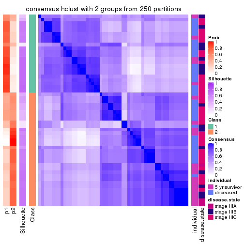
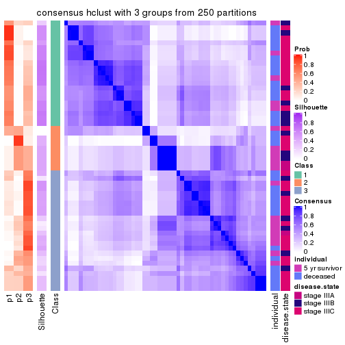
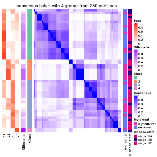
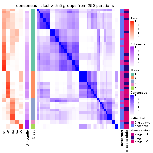
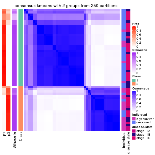
Heatmaps for the consensus matrix. It visualizes the probability of two samples to be in a same group.
consensus_heatmap(res, k = 2)
consensus_heatmap(res, k = 3)
consensus_heatmap(res, k = 4)
consensus_heatmap(res, k = 5)
consensus_heatmap(res, k = 6)
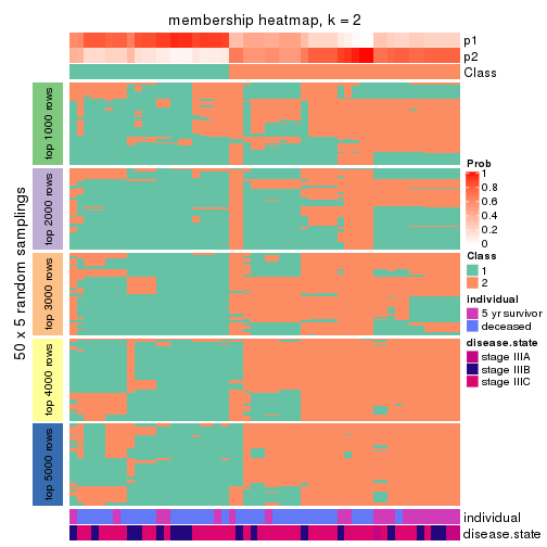
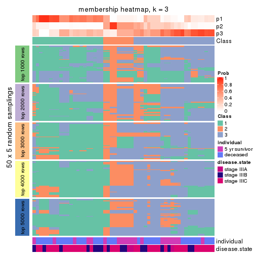
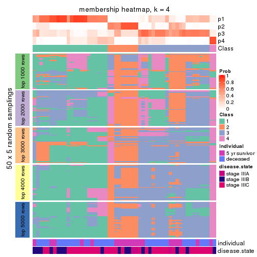
Heatmaps for the membership of samples in all partitions to see how consistent they are:
membership_heatmap(res, k = 2)
membership_heatmap(res, k = 3)
membership_heatmap(res, k = 4)
membership_heatmap(res, k = 5)
membership_heatmap(res, k = 6)
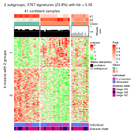
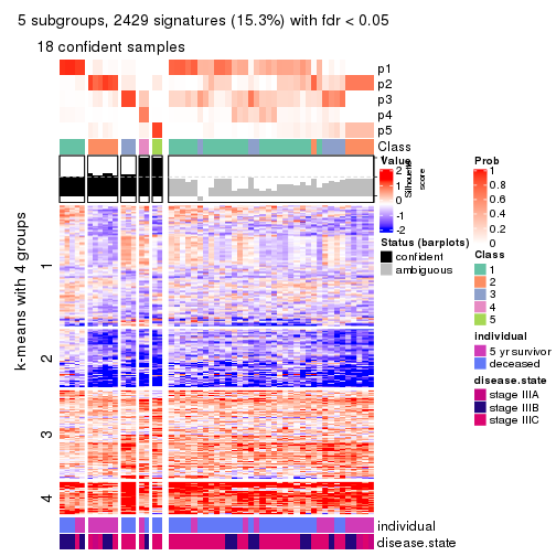
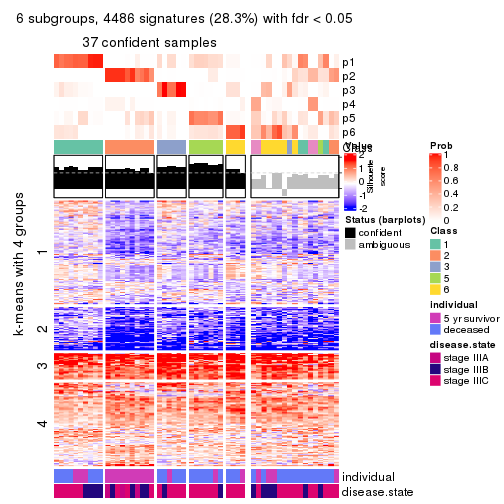
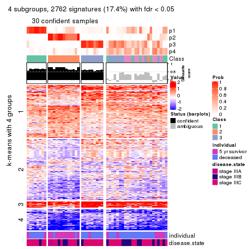
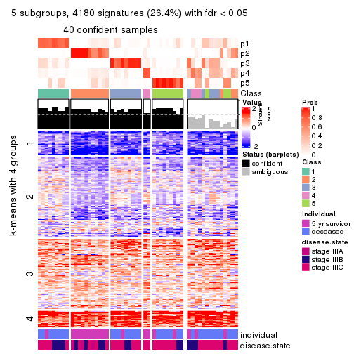
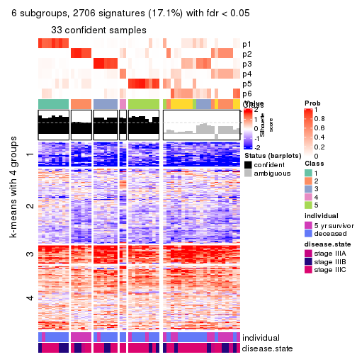
As soon as we have had the classes for columns, we can look for signatures which are significantly different between classes which can be candidate marks for certain classes. Following are the heatmaps for signatures.
Signature heatmaps where rows are scaled:
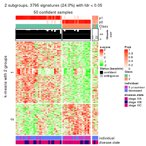
get_signatures(res, k = 2)
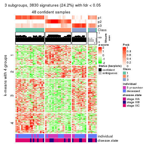
get_signatures(res, k = 3)

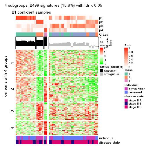
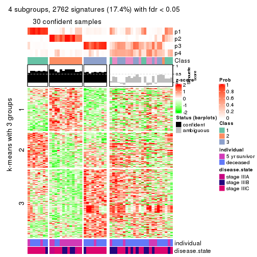
get_signatures(res, k = 4)
get_signatures(res, k = 5)
get_signatures(res, k = 6)
Signature heatmaps where rows are not scaled:
get_signatures(res, k = 2, scale_rows = FALSE)
get_signatures(res, k = 3, scale_rows = FALSE)

get_signatures(res, k = 4, scale_rows = FALSE)
get_signatures(res, k = 5, scale_rows = FALSE)
get_signatures(res, k = 6, scale_rows = FALSE)
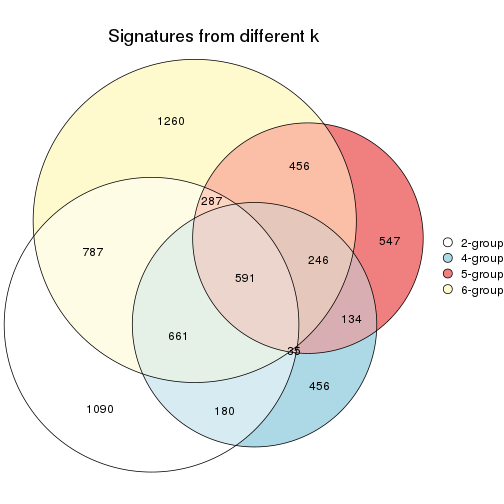
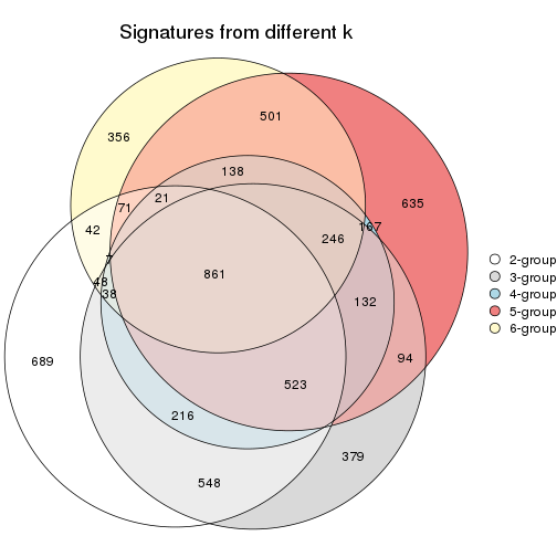
Compare the overlap of signatures from different k:
compare_signatures(res)
get_signature() returns a data frame invisibly. TO get the list of signatures, the function
call should be assigned to a variable explicitly. In following code, if plot argument is set
to FALSE, no heatmap is plotted while only the differential analysis is performed.
# code only for demonstration
tb = get_signature(res, k = ..., plot = FALSE)
An example of the output of tb is:
#>   which_row         fdr    mean_1    mean_2 scaled_mean_1 scaled_mean_2 km
#> 1        38 0.042760348  8.373488  9.131774    -0.5533452     0.5164555  1
#> 2        40 0.018707592  7.106213  8.469186    -0.6173731     0.5762149  1
#> 3        55 0.019134737 10.221463 11.207825    -0.6159697     0.5749050  1
#> 4        59 0.006059896  5.921854  7.869574    -0.6899429     0.6439467  1
#> 5        60 0.018055526  8.928898 10.211722    -0.6204761     0.5791110  1
#> 6        98 0.009384629 15.714769 14.887706     0.6635654    -0.6193277  2
...
The columns in tb are:
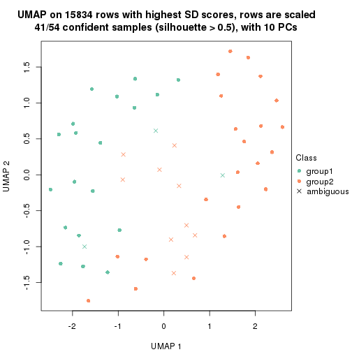
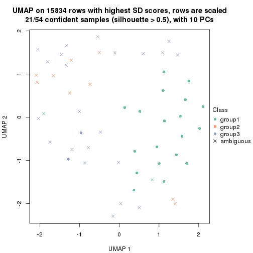
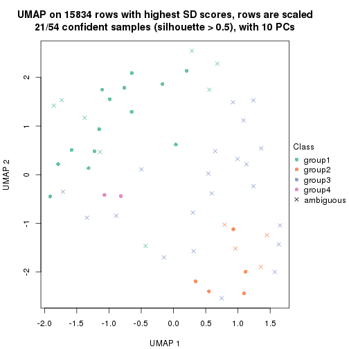
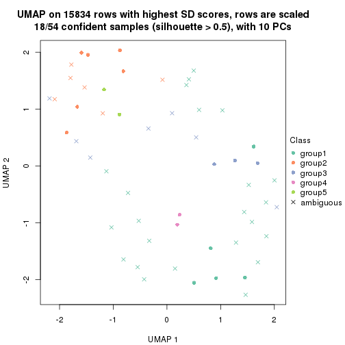
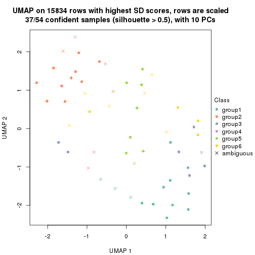
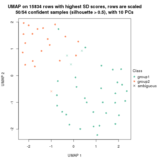
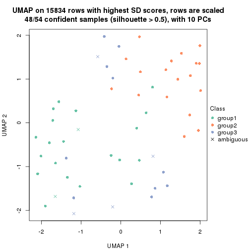
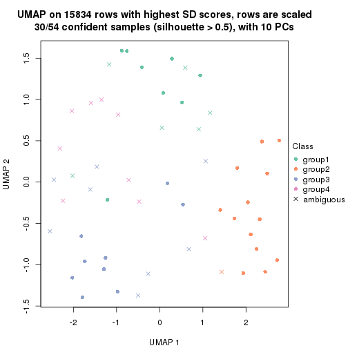
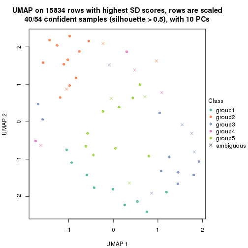
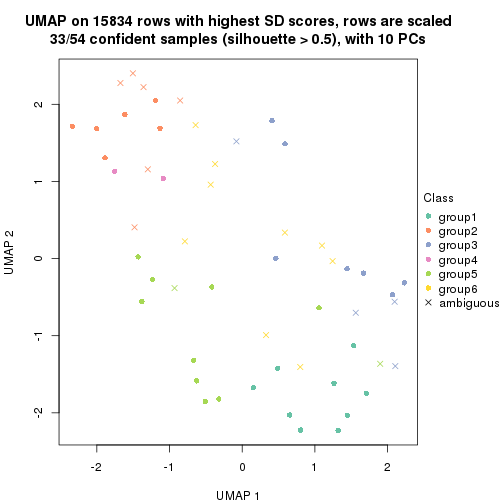
which_row: row indices corresponding to the input matrix.fdr: FDR for the differential test. mean_x: The mean value in group x.scaled_mean_x: The mean value in group x after rows are scaled.km: Row groups if k-means clustering is applied to rows.UMAP plot which shows how samples are separated.
dimension_reduction(res, k = 2, method = "UMAP")
dimension_reduction(res, k = 3, method = "UMAP")
dimension_reduction(res, k = 4, method = "UMAP")
dimension_reduction(res, k = 5, method = "UMAP")
dimension_reduction(res, k = 6, method = "UMAP")
Following heatmap shows how subgroups are split when increasing k:
collect_classes(res)
Test correlation between subgroups and known annotations. If the known annotation is numeric, one-way ANOVA test is applied, and if the known annotation is discrete, chi-squared contingency table test is applied.
test_to_known_factors(res)
#>            n individual(p) disease.state(p) k
#> SD:hclust 41      0.031757           0.2472 2
#> SD:hclust 21      0.966852           0.9064 3
#> SD:hclust 21      0.023042           0.0960 4
#> SD:hclust 18      0.024406           0.3266 5
#> SD:hclust 37      0.000985           0.0687 6
If matrix rows can be associated to genes, consider to use functional_enrichment(res,
...) to perform function enrichment for the signature genes. See this vignette for more detailed explanations.
The object with results only for a single top-value method and a single partition method can be extracted as:
res = res_list["SD", "kmeans"]
# you can also extract it by
# res = res_list["SD:kmeans"]
A summary of res and all the functions that can be applied to it:
res
#> A 'ConsensusPartition' object with k = 2, 3, 4, 5, 6.
#>   On a matrix with 15834 rows and 54 columns.
#>   Top rows (1000, 2000, 3000, 4000, 5000) are extracted by 'SD' method.
#>   Subgroups are detected by 'kmeans' method.
#>   Performed in total 1250 partitions by row resampling.
#>   Best k for subgroups seems to be 2.
#>
#> Following methods can be applied to this 'ConsensusPartition' object:
#>  [1] "cola_report"             "collect_classes"         "collect_plots"
#>  [4] "collect_stats"           "colnames"                "compare_signatures"
#>  [7] "consensus_heatmap"       "dimension_reduction"     "functional_enrichment"
#> [10] "get_anno_col"            "get_anno"                "get_classes"
#> [13] "get_consensus"           "get_matrix"              "get_membership"
#> [16] "get_param"               "get_signatures"          "get_stats"
#> [19] "is_best_k"               "is_stable_k"             "membership_heatmap"
#> [22] "ncol"                    "nrow"                    "plot_ecdf"
#> [25] "rownames"                "select_partition_number" "show"
#> [28] "suggest_best_k"          "test_to_known_factors"
collect_plots() function collects all the plots made from res for all k (number of partitions)
into one single page to provide an easy and fast comparison between different k.
collect_plots(res)
The plots are:
k and the heatmap of
predicted classes for each k.k.k.k.All the plots in panels can be made by individual functions and they are plotted later in this section.
select_partition_number() produces several plots showing different
statistics for choosing “optimized” k. There are following statistics:
k;k, the area increased is defined as \(A_k - A_{k-1}\).The detailed explanations of these statistics can be found in the cola vignette.
Generally speaking, lower PAC score, higher mean silhouette score or higher
concordance corresponds to better partition. Rand index and Jaccard index
measure how similar the current partition is compared to partition with k-1.
If they are too similar, we won't accept k is better than k-1.
select_partition_number(res)
The numeric values for all these statistics can be obtained by get_stats().
get_stats(res)
#>   k 1-PAC mean_silhouette concordance area_increased  Rand Jaccard
#> 2 2 0.714           0.845       0.925         0.4814 0.525   0.525
#> 3 3 0.411           0.644       0.770         0.3543 0.774   0.582
#> 4 4 0.526           0.469       0.664         0.1390 0.837   0.561
#> 5 5 0.636           0.576       0.758         0.0718 0.925   0.714
#> 6 6 0.704           0.507       0.685         0.0422 0.921   0.655
suggest_best_k() suggests the best \(k\) based on these statistics. The rules are as follows:
suggest_best_k(res)
#> [1] 2
Following shows the table of the partitions (You need to click the show/hide
code output link to see it). The membership matrix (columns with name p*)
is inferred by
clue::cl_consensus()
function with the SE method. Basically the value in the membership matrix
represents the probability to belong to a certain group. The finall class
label for an item is determined with the group with highest probability it
belongs to.
In get_classes() function, the entropy is calculated from the membership
matrix and the silhouette score is calculated from the consensus matrix.
cbind(get_classes(res, k = 2), get_membership(res, k = 2))
#>           class entropy silhouette    p1    p2
#> GSM311939     2  0.2236      0.927 0.036 0.964
#> GSM311963     2  0.2236      0.927 0.036 0.964
#> GSM311973     2  0.0938      0.920 0.012 0.988
#> GSM311940     2  0.2043      0.926 0.032 0.968
#> GSM311953     2  0.0938      0.923 0.012 0.988
#> GSM311974     2  0.0938      0.920 0.012 0.988
#> GSM311975     1  0.0938      0.916 0.988 0.012
#> GSM311977     2  0.2236      0.927 0.036 0.964
#> GSM311982     1  0.2043      0.910 0.968 0.032
#> GSM311990     2  0.2043      0.926 0.032 0.968
#> GSM311943     1  0.0938      0.918 0.988 0.012
#> GSM311944     1  0.2043      0.910 0.968 0.032
#> GSM311946     2  0.1414      0.925 0.020 0.980
#> GSM311956     2  0.0938      0.920 0.012 0.988
#> GSM311967     2  0.6148      0.816 0.152 0.848
#> GSM311968     2  0.5946      0.795 0.144 0.856
#> GSM311972     1  0.1414      0.914 0.980 0.020
#> GSM311980     2  0.0938      0.920 0.012 0.988
#> GSM311981     1  0.1633      0.911 0.976 0.024
#> GSM311988     2  0.2236      0.927 0.036 0.964
#> GSM311957     1  0.2236      0.908 0.964 0.036
#> GSM311960     2  0.9996     -0.117 0.488 0.512
#> GSM311971     1  0.6623      0.789 0.828 0.172
#> GSM311976     1  0.0672      0.917 0.992 0.008
#> GSM311978     1  0.1414      0.914 0.980 0.020
#> GSM311979     1  0.2043      0.910 0.968 0.032
#> GSM311983     1  0.0672      0.918 0.992 0.008
#> GSM311986     1  0.8861      0.558 0.696 0.304
#> GSM311991     1  0.0938      0.916 0.988 0.012
#> GSM311938     2  0.7376      0.746 0.208 0.792
#> GSM311941     1  0.0376      0.918 0.996 0.004
#> GSM311942     1  0.9833      0.348 0.576 0.424
#> GSM311945     1  0.2043      0.910 0.968 0.032
#> GSM311947     2  0.2236      0.925 0.036 0.964
#> GSM311948     2  0.0938      0.920 0.012 0.988
#> GSM311949     1  0.1414      0.914 0.980 0.020
#> GSM311950     2  0.2043      0.926 0.032 0.968
#> GSM311951     1  0.9833      0.348 0.576 0.424
#> GSM311952     1  0.0938      0.918 0.988 0.012
#> GSM311954     1  0.1633      0.911 0.976 0.024
#> GSM311955     1  0.0938      0.916 0.988 0.012
#> GSM311958     1  0.0938      0.916 0.988 0.012
#> GSM311959     1  0.0938      0.916 0.988 0.012
#> GSM311961     1  0.0938      0.918 0.988 0.012
#> GSM311962     1  0.0672      0.917 0.992 0.008
#> GSM311964     1  0.1414      0.914 0.980 0.020
#> GSM311965     1  0.9795      0.371 0.584 0.416
#> GSM311966     1  0.0672      0.917 0.992 0.008
#> GSM311969     1  0.0938      0.918 0.988 0.012
#> GSM311970     2  0.1633      0.927 0.024 0.976
#> GSM311984     1  0.0672      0.918 0.992 0.008
#> GSM311985     1  0.0376      0.918 0.996 0.004
#> GSM311987     1  0.7453      0.716 0.788 0.212
#> GSM311989     1  0.6623      0.789 0.828 0.172
cbind(get_classes(res, k = 3), get_membership(res, k = 3))
#>           class entropy silhouette    p1    p2    p3
#> GSM311939     2  0.0000      0.815 0.000 1.000 0.000
#> GSM311963     2  0.0000      0.815 0.000 1.000 0.000
#> GSM311973     2  0.5591      0.642 0.000 0.696 0.304
#> GSM311940     2  0.0237      0.815 0.000 0.996 0.004
#> GSM311953     2  0.2878      0.805 0.000 0.904 0.096
#> GSM311974     2  0.3482      0.796 0.000 0.872 0.128
#> GSM311975     1  0.5158      0.605 0.764 0.004 0.232
#> GSM311977     2  0.0000      0.815 0.000 1.000 0.000
#> GSM311982     3  0.5591      0.558 0.304 0.000 0.696
#> GSM311990     2  0.8349      0.655 0.128 0.608 0.264
#> GSM311943     1  0.5873      0.695 0.684 0.004 0.312
#> GSM311944     3  0.4452      0.604 0.192 0.000 0.808
#> GSM311946     2  0.2878      0.805 0.000 0.904 0.096
#> GSM311956     2  0.4235      0.772 0.000 0.824 0.176
#> GSM311967     2  0.8938      0.516 0.284 0.552 0.164
#> GSM311968     3  0.4784      0.507 0.004 0.200 0.796
#> GSM311972     1  0.4399      0.711 0.812 0.000 0.188
#> GSM311980     2  0.4346      0.767 0.000 0.816 0.184
#> GSM311981     1  0.5974      0.506 0.784 0.068 0.148
#> GSM311988     2  0.0000      0.815 0.000 1.000 0.000
#> GSM311957     3  0.5687      0.588 0.224 0.020 0.756
#> GSM311960     3  0.3670      0.683 0.020 0.092 0.888
#> GSM311971     3  0.8212      0.465 0.360 0.084 0.556
#> GSM311976     1  0.5058      0.650 0.756 0.000 0.244
#> GSM311978     1  0.5810      0.490 0.664 0.000 0.336
#> GSM311979     3  0.6154      0.365 0.408 0.000 0.592
#> GSM311983     1  0.5365      0.722 0.744 0.004 0.252
#> GSM311986     1  0.8848      0.438 0.560 0.156 0.284
#> GSM311991     1  0.2584      0.607 0.928 0.008 0.064
#> GSM311938     2  0.5461      0.657 0.244 0.748 0.008
#> GSM311941     3  0.6495     -0.177 0.460 0.004 0.536
#> GSM311942     3  0.2383      0.704 0.016 0.044 0.940
#> GSM311945     3  0.2356      0.699 0.072 0.000 0.928
#> GSM311947     2  0.9329      0.561 0.180 0.488 0.332
#> GSM311948     2  0.6154      0.523 0.000 0.592 0.408
#> GSM311949     1  0.5497      0.593 0.708 0.000 0.292
#> GSM311950     2  0.5507      0.745 0.136 0.808 0.056
#> GSM311951     3  0.2527      0.705 0.020 0.044 0.936
#> GSM311952     1  0.5722      0.705 0.704 0.004 0.292
#> GSM311954     1  0.6906      0.596 0.724 0.084 0.192
#> GSM311955     1  0.4834      0.739 0.792 0.004 0.204
#> GSM311958     1  0.4555      0.742 0.800 0.000 0.200
#> GSM311959     1  0.4733      0.662 0.800 0.004 0.196
#> GSM311961     1  0.5404      0.720 0.740 0.004 0.256
#> GSM311962     1  0.4233      0.733 0.836 0.004 0.160
#> GSM311964     3  0.6260      0.306 0.448 0.000 0.552
#> GSM311965     3  0.3234      0.694 0.020 0.072 0.908
#> GSM311966     1  0.4346      0.713 0.816 0.000 0.184
#> GSM311969     1  0.5929      0.685 0.676 0.004 0.320
#> GSM311970     2  0.4095      0.781 0.064 0.880 0.056
#> GSM311984     1  0.5517      0.720 0.728 0.004 0.268
#> GSM311985     1  0.4346      0.713 0.816 0.000 0.184
#> GSM311987     1  0.7762      0.518 0.668 0.120 0.212
#> GSM311989     3  0.2434      0.707 0.024 0.036 0.940
cbind(get_classes(res, k = 4), get_membership(res, k = 4))
#>           class entropy silhouette    p1    p2    p3    p4
#> GSM311939     2  0.0469    0.79464 0.000 0.988 0.000 0.012
#> GSM311963     2  0.0469    0.79464 0.000 0.988 0.000 0.012
#> GSM311973     2  0.5890    0.62833 0.268 0.660 0.000 0.072
#> GSM311940     2  0.0469    0.79464 0.000 0.988 0.000 0.012
#> GSM311953     2  0.3354    0.77350 0.084 0.872 0.000 0.044
#> GSM311974     2  0.5188    0.67954 0.240 0.716 0.000 0.044
#> GSM311975     3  0.4988    0.39454 0.020 0.000 0.692 0.288
#> GSM311977     2  0.0469    0.79464 0.000 0.988 0.000 0.012
#> GSM311982     1  0.6915    0.07265 0.564 0.000 0.140 0.296
#> GSM311990     1  0.7798    0.22161 0.468 0.200 0.008 0.324
#> GSM311943     3  0.1792    0.62180 0.068 0.000 0.932 0.000
#> GSM311944     1  0.3626    0.57900 0.812 0.000 0.184 0.004
#> GSM311946     2  0.3149    0.77579 0.088 0.880 0.000 0.032
#> GSM311956     2  0.5498    0.64793 0.272 0.680 0.000 0.048
#> GSM311967     4  0.8212   -0.08089 0.032 0.220 0.252 0.496
#> GSM311968     1  0.2613    0.66700 0.916 0.024 0.008 0.052
#> GSM311972     3  0.6323   -0.11703 0.060 0.000 0.500 0.440
#> GSM311980     2  0.5646    0.64413 0.272 0.672 0.000 0.056
#> GSM311981     4  0.5626   -0.11644 0.012 0.020 0.324 0.644
#> GSM311988     2  0.0469    0.79464 0.000 0.988 0.000 0.012
#> GSM311957     1  0.6308    0.35407 0.656 0.000 0.208 0.136
#> GSM311960     1  0.2586    0.67078 0.912 0.008 0.012 0.068
#> GSM311971     4  0.8664    0.32687 0.336 0.044 0.216 0.404
#> GSM311976     4  0.6621    0.27357 0.084 0.000 0.408 0.508
#> GSM311978     4  0.7110    0.32413 0.128 0.000 0.412 0.460
#> GSM311979     4  0.7785    0.35007 0.348 0.000 0.248 0.404
#> GSM311983     3  0.1629    0.60971 0.024 0.000 0.952 0.024
#> GSM311986     3  0.6515    0.49055 0.084 0.048 0.700 0.168
#> GSM311991     4  0.4888   -0.17599 0.000 0.000 0.412 0.588
#> GSM311938     2  0.6596    0.43709 0.004 0.628 0.120 0.248
#> GSM311941     1  0.7200   -0.02362 0.484 0.000 0.372 0.144
#> GSM311942     1  0.0779    0.68808 0.980 0.000 0.016 0.004
#> GSM311945     1  0.2335    0.67156 0.920 0.000 0.020 0.060
#> GSM311947     1  0.7269    0.29474 0.480 0.116 0.008 0.396
#> GSM311948     1  0.5754    0.22749 0.636 0.316 0.000 0.048
#> GSM311949     4  0.6998    0.31144 0.116 0.000 0.416 0.468
#> GSM311950     2  0.5130    0.58811 0.020 0.668 0.000 0.312
#> GSM311951     1  0.0707    0.68803 0.980 0.000 0.020 0.000
#> GSM311952     3  0.1902    0.62146 0.064 0.000 0.932 0.004
#> GSM311954     3  0.6725    0.48479 0.052 0.036 0.616 0.296
#> GSM311955     3  0.4337    0.60421 0.052 0.000 0.808 0.140
#> GSM311958     3  0.4224    0.59730 0.044 0.000 0.812 0.144
#> GSM311959     3  0.5801    0.52317 0.052 0.004 0.664 0.280
#> GSM311961     3  0.1733    0.61065 0.028 0.000 0.948 0.024
#> GSM311962     3  0.4283    0.35773 0.004 0.000 0.740 0.256
#> GSM311964     4  0.7680    0.38432 0.324 0.000 0.232 0.444
#> GSM311965     1  0.1509    0.68503 0.960 0.008 0.012 0.020
#> GSM311966     3  0.5459    0.00932 0.016 0.000 0.552 0.432
#> GSM311969     3  0.2596    0.62033 0.068 0.000 0.908 0.024
#> GSM311970     2  0.4610    0.66551 0.020 0.744 0.000 0.236
#> GSM311984     3  0.1388    0.61568 0.028 0.000 0.960 0.012
#> GSM311985     3  0.6060   -0.06740 0.044 0.000 0.516 0.440
#> GSM311987     3  0.7048    0.45948 0.064 0.040 0.592 0.304
#> GSM311989     1  0.2089    0.67627 0.932 0.000 0.020 0.048
cbind(get_classes(res, k = 5), get_membership(res, k = 5))
#>           class entropy silhouette    p1    p2    p3    p4    p5
#> GSM311939     2  0.0404     0.7111 0.000 0.988 0.000 0.012 0.000
#> GSM311963     2  0.0404     0.7111 0.000 0.988 0.000 0.012 0.000
#> GSM311973     2  0.6905     0.5908 0.100 0.584 0.000 0.108 0.208
#> GSM311940     2  0.0404     0.7111 0.000 0.988 0.000 0.012 0.000
#> GSM311953     2  0.4299     0.6953 0.068 0.808 0.000 0.084 0.040
#> GSM311974     2  0.6030     0.6470 0.084 0.680 0.000 0.096 0.140
#> GSM311975     3  0.4067     0.4138 0.000 0.000 0.692 0.300 0.008
#> GSM311977     2  0.0404     0.7111 0.000 0.988 0.000 0.012 0.000
#> GSM311982     5  0.5322     0.1642 0.372 0.000 0.036 0.012 0.580
#> GSM311990     4  0.6169     0.3245 0.012 0.080 0.004 0.484 0.420
#> GSM311943     3  0.0955     0.7086 0.004 0.000 0.968 0.000 0.028
#> GSM311944     5  0.2295     0.6944 0.004 0.000 0.088 0.008 0.900
#> GSM311946     2  0.4123     0.6979 0.056 0.820 0.000 0.080 0.044
#> GSM311956     2  0.6819     0.5916 0.088 0.588 0.000 0.108 0.216
#> GSM311967     4  0.4366     0.5672 0.008 0.092 0.068 0.808 0.024
#> GSM311968     5  0.2954     0.6422 0.064 0.004 0.000 0.056 0.876
#> GSM311972     1  0.4429     0.7260 0.744 0.000 0.192 0.064 0.000
#> GSM311980     2  0.6844     0.5877 0.088 0.584 0.000 0.108 0.220
#> GSM311981     4  0.4022     0.5497 0.100 0.000 0.092 0.804 0.004
#> GSM311988     2  0.0404     0.7111 0.000 0.988 0.000 0.012 0.000
#> GSM311957     5  0.5797     0.5362 0.204 0.000 0.092 0.036 0.668
#> GSM311960     5  0.2299     0.7296 0.052 0.000 0.004 0.032 0.912
#> GSM311971     1  0.4810     0.6224 0.712 0.020 0.024 0.004 0.240
#> GSM311976     1  0.3404     0.7851 0.840 0.000 0.124 0.024 0.012
#> GSM311978     1  0.3732     0.7849 0.816 0.000 0.144 0.016 0.024
#> GSM311979     1  0.4351     0.6344 0.724 0.000 0.028 0.004 0.244
#> GSM311983     3  0.1393     0.7079 0.024 0.000 0.956 0.012 0.008
#> GSM311986     3  0.4352     0.5854 0.000 0.036 0.792 0.132 0.040
#> GSM311991     4  0.5116     0.4329 0.120 0.000 0.188 0.692 0.000
#> GSM311938     2  0.6965     0.0625 0.144 0.524 0.048 0.284 0.000
#> GSM311941     5  0.7525     0.0450 0.300 0.000 0.208 0.056 0.436
#> GSM311942     5  0.0486     0.7338 0.004 0.000 0.004 0.004 0.988
#> GSM311945     5  0.2201     0.7334 0.040 0.000 0.008 0.032 0.920
#> GSM311947     4  0.4833     0.3782 0.000 0.024 0.000 0.564 0.412
#> GSM311948     5  0.6659     0.2302 0.076 0.244 0.000 0.092 0.588
#> GSM311949     1  0.3694     0.7867 0.824 0.000 0.132 0.024 0.020
#> GSM311950     2  0.5099     0.0687 0.028 0.528 0.004 0.440 0.000
#> GSM311951     5  0.0486     0.7338 0.004 0.000 0.004 0.004 0.988
#> GSM311952     3  0.1117     0.7104 0.020 0.000 0.964 0.000 0.016
#> GSM311954     3  0.7277     0.2943 0.164 0.012 0.420 0.380 0.024
#> GSM311955     3  0.4523     0.6459 0.148 0.000 0.768 0.072 0.012
#> GSM311958     3  0.5338     0.6070 0.180 0.000 0.696 0.112 0.012
#> GSM311959     3  0.6899     0.3311 0.160 0.000 0.448 0.368 0.024
#> GSM311961     3  0.1588     0.7050 0.028 0.000 0.948 0.016 0.008
#> GSM311962     3  0.4546     0.4820 0.304 0.000 0.668 0.028 0.000
#> GSM311964     1  0.4565     0.6327 0.720 0.000 0.024 0.016 0.240
#> GSM311965     5  0.0727     0.7311 0.004 0.000 0.004 0.012 0.980
#> GSM311966     1  0.4134     0.7335 0.760 0.000 0.196 0.044 0.000
#> GSM311969     3  0.0955     0.7086 0.004 0.000 0.968 0.000 0.028
#> GSM311970     2  0.5421     0.3569 0.060 0.612 0.008 0.320 0.000
#> GSM311984     3  0.1393     0.7079 0.024 0.000 0.956 0.012 0.008
#> GSM311985     1  0.4429     0.7204 0.744 0.000 0.192 0.064 0.000
#> GSM311987     3  0.7312     0.2767 0.144 0.016 0.420 0.392 0.028
#> GSM311989     5  0.2122     0.7339 0.036 0.000 0.008 0.032 0.924
cbind(get_classes(res, k = 6), get_membership(res, k = 6))
#>           class entropy silhouette    p1    p2    p3    p4    p5    p6
#> GSM311939     2  0.3797     0.3309 0.000 0.580 0.000 0.420 0.000 0.000
#> GSM311963     2  0.3797     0.3309 0.000 0.580 0.000 0.420 0.000 0.000
#> GSM311973     2  0.3059     0.5172 0.004 0.848 0.000 0.040 0.104 0.004
#> GSM311940     2  0.3797     0.3309 0.000 0.580 0.000 0.420 0.000 0.000
#> GSM311953     2  0.0935     0.5470 0.000 0.964 0.000 0.032 0.004 0.000
#> GSM311974     2  0.0935     0.5461 0.000 0.964 0.000 0.004 0.032 0.000
#> GSM311975     3  0.4323     0.3606 0.004 0.000 0.600 0.020 0.000 0.376
#> GSM311977     2  0.3797     0.3309 0.000 0.580 0.000 0.420 0.000 0.000
#> GSM311982     5  0.5057     0.0644 0.412 0.000 0.016 0.044 0.528 0.000
#> GSM311990     6  0.7334     0.0756 0.000 0.092 0.008 0.204 0.316 0.380
#> GSM311943     3  0.0767     0.7354 0.012 0.000 0.976 0.008 0.004 0.000
#> GSM311944     5  0.2479     0.7321 0.028 0.000 0.064 0.016 0.892 0.000
#> GSM311946     2  0.1349     0.5424 0.000 0.940 0.000 0.056 0.004 0.000
#> GSM311956     2  0.2917     0.5163 0.000 0.852 0.000 0.040 0.104 0.004
#> GSM311967     6  0.3952     0.1628 0.000 0.008 0.024 0.224 0.004 0.740
#> GSM311968     5  0.2915     0.6680 0.000 0.164 0.004 0.004 0.824 0.004
#> GSM311972     1  0.4379     0.6979 0.752 0.000 0.040 0.028 0.008 0.172
#> GSM311980     2  0.3059     0.5172 0.004 0.848 0.000 0.040 0.104 0.004
#> GSM311981     6  0.4463     0.2394 0.044 0.000 0.036 0.188 0.000 0.732
#> GSM311988     2  0.3797     0.3309 0.000 0.580 0.000 0.420 0.000 0.000
#> GSM311957     5  0.6115     0.5182 0.232 0.000 0.060 0.076 0.608 0.024
#> GSM311960     5  0.2732     0.7578 0.028 0.004 0.000 0.060 0.884 0.024
#> GSM311971     1  0.3376     0.7439 0.820 0.004 0.008 0.032 0.136 0.000
#> GSM311976     1  0.1710     0.8081 0.936 0.000 0.016 0.000 0.028 0.020
#> GSM311978     1  0.2081     0.8056 0.916 0.000 0.036 0.036 0.012 0.000
#> GSM311979     1  0.3351     0.7419 0.820 0.000 0.016 0.028 0.136 0.000
#> GSM311983     3  0.2762     0.7181 0.016 0.000 0.884 0.056 0.008 0.036
#> GSM311986     3  0.2838     0.6228 0.000 0.000 0.852 0.028 0.004 0.116
#> GSM311991     6  0.5195     0.1980 0.068 0.000 0.056 0.200 0.000 0.676
#> GSM311938     6  0.7774    -0.2159 0.096 0.268 0.028 0.252 0.000 0.356
#> GSM311941     5  0.7617     0.0235 0.268 0.000 0.152 0.016 0.404 0.160
#> GSM311942     5  0.0692     0.7694 0.000 0.020 0.000 0.004 0.976 0.000
#> GSM311945     5  0.1991     0.7689 0.012 0.000 0.000 0.044 0.920 0.024
#> GSM311947     6  0.6687     0.0996 0.000 0.052 0.000 0.200 0.304 0.444
#> GSM311948     2  0.4284     0.1802 0.000 0.608 0.004 0.012 0.372 0.004
#> GSM311949     1  0.1630     0.8086 0.940 0.000 0.024 0.000 0.020 0.016
#> GSM311950     4  0.5620     0.7204 0.016 0.148 0.000 0.588 0.000 0.248
#> GSM311951     5  0.0547     0.7702 0.000 0.020 0.000 0.000 0.980 0.000
#> GSM311952     3  0.0748     0.7360 0.016 0.000 0.976 0.004 0.004 0.000
#> GSM311954     6  0.5952     0.1373 0.108 0.000 0.364 0.024 0.004 0.500
#> GSM311955     3  0.4664     0.4850 0.116 0.000 0.696 0.004 0.000 0.184
#> GSM311958     3  0.5394     0.3913 0.128 0.000 0.616 0.008 0.004 0.244
#> GSM311959     6  0.5673     0.1018 0.108 0.000 0.384 0.008 0.004 0.496
#> GSM311961     3  0.3172     0.7078 0.020 0.000 0.860 0.064 0.008 0.048
#> GSM311962     3  0.5451     0.4326 0.256 0.000 0.596 0.004 0.004 0.140
#> GSM311964     1  0.2790     0.7487 0.840 0.000 0.000 0.020 0.140 0.000
#> GSM311965     5  0.1211     0.7653 0.004 0.024 0.004 0.004 0.960 0.004
#> GSM311966     1  0.4060     0.7171 0.780 0.000 0.040 0.028 0.004 0.148
#> GSM311969     3  0.0767     0.7354 0.012 0.000 0.976 0.008 0.004 0.000
#> GSM311970     4  0.5783     0.6926 0.020 0.260 0.000 0.568 0.000 0.152
#> GSM311984     3  0.2882     0.7165 0.016 0.000 0.876 0.064 0.008 0.036
#> GSM311985     1  0.4277     0.7024 0.764 0.000 0.040 0.028 0.008 0.160
#> GSM311987     6  0.5952     0.1373 0.108 0.000 0.364 0.024 0.004 0.500
#> GSM311989     5  0.2228     0.7659 0.008 0.004 0.000 0.056 0.908 0.024
Heatmaps for the consensus matrix. It visualizes the probability of two samples to be in a same group.
consensus_heatmap(res, k = 2)
consensus_heatmap(res, k = 3)
consensus_heatmap(res, k = 4)
consensus_heatmap(res, k = 5)
consensus_heatmap(res, k = 6)
Heatmaps for the membership of samples in all partitions to see how consistent they are:
membership_heatmap(res, k = 2)
membership_heatmap(res, k = 3)
membership_heatmap(res, k = 4)
membership_heatmap(res, k = 5)
membership_heatmap(res, k = 6)
As soon as we have had the classes for columns, we can look for signatures which are significantly different between classes which can be candidate marks for certain classes. Following are the heatmaps for signatures.
Signature heatmaps where rows are scaled:
get_signatures(res, k = 2)
get_signatures(res, k = 3)
get_signatures(res, k = 4)
get_signatures(res, k = 5)
get_signatures(res, k = 6)
Signature heatmaps where rows are not scaled:
get_signatures(res, k = 2, scale_rows = FALSE)
get_signatures(res, k = 3, scale_rows = FALSE)
get_signatures(res, k = 4, scale_rows = FALSE)
get_signatures(res, k = 5, scale_rows = FALSE)
get_signatures(res, k = 6, scale_rows = FALSE)
Compare the overlap of signatures from different k:
compare_signatures(res)
get_signature() returns a data frame invisibly. TO get the list of signatures, the function
call should be assigned to a variable explicitly. In following code, if plot argument is set
to FALSE, no heatmap is plotted while only the differential analysis is performed.
# code only for demonstration
tb = get_signature(res, k = ..., plot = FALSE)
An example of the output of tb is:
#>   which_row         fdr    mean_1    mean_2 scaled_mean_1 scaled_mean_2 km
#> 1        38 0.042760348  8.373488  9.131774    -0.5533452     0.5164555  1
#> 2        40 0.018707592  7.106213  8.469186    -0.6173731     0.5762149  1
#> 3        55 0.019134737 10.221463 11.207825    -0.6159697     0.5749050  1
#> 4        59 0.006059896  5.921854  7.869574    -0.6899429     0.6439467  1
#> 5        60 0.018055526  8.928898 10.211722    -0.6204761     0.5791110  1
#> 6        98 0.009384629 15.714769 14.887706     0.6635654    -0.6193277  2
...
The columns in tb are:
which_row: row indices corresponding to the input matrix.fdr: FDR for the differential test. mean_x: The mean value in group x.scaled_mean_x: The mean value in group x after rows are scaled.km: Row groups if k-means clustering is applied to rows.UMAP plot which shows how samples are separated.
dimension_reduction(res, k = 2, method = "UMAP")
dimension_reduction(res, k = 3, method = "UMAP")
dimension_reduction(res, k = 4, method = "UMAP")
dimension_reduction(res, k = 5, method = "UMAP")
dimension_reduction(res, k = 6, method = "UMAP")
Following heatmap shows how subgroups are split when increasing k:
collect_classes(res)
Test correlation between subgroups and known annotations. If the known annotation is numeric, one-way ANOVA test is applied, and if the known annotation is discrete, chi-squared contingency table test is applied.
test_to_known_factors(res)
#>            n individual(p) disease.state(p) k
#> SD:kmeans 50      4.50e-04           0.0738 2
#> SD:kmeans 48      3.45e-03           0.1860 3
#> SD:kmeans 30      1.11e-03           0.1296 4
#> SD:kmeans 40      2.68e-05           0.1494 5
#> SD:kmeans 33      1.64e-03           0.5519 6
If matrix rows can be associated to genes, consider to use functional_enrichment(res,
...) to perform function enrichment for the signature genes. See this vignette for more detailed explanations.
The object with results only for a single top-value method and a single partition method can be extracted as:
res = res_list["SD", "skmeans"]
# you can also extract it by
# res = res_list["SD:skmeans"]
A summary of res and all the functions that can be applied to it:
res
#> A 'ConsensusPartition' object with k = 2, 3, 4, 5, 6.
#>   On a matrix with 15834 rows and 54 columns.
#>   Top rows (1000, 2000, 3000, 4000, 5000) are extracted by 'SD' method.
#>   Subgroups are detected by 'skmeans' method.
#>   Performed in total 1250 partitions by row resampling.
#>   Best k for subgroups seems to be 2.
#>
#> Following methods can be applied to this 'ConsensusPartition' object:
#>  [1] "cola_report"             "collect_classes"         "collect_plots"
#>  [4] "collect_stats"           "colnames"                "compare_signatures"
#>  [7] "consensus_heatmap"       "dimension_reduction"     "functional_enrichment"
#> [10] "get_anno_col"            "get_anno"                "get_classes"
#> [13] "get_consensus"           "get_matrix"              "get_membership"
#> [16] "get_param"               "get_signatures"          "get_stats"
#> [19] "is_best_k"               "is_stable_k"             "membership_heatmap"
#> [22] "ncol"                    "nrow"                    "plot_ecdf"
#> [25] "rownames"                "select_partition_number" "show"
#> [28] "suggest_best_k"          "test_to_known_factors"
collect_plots() function collects all the plots made from res for all k (number of partitions)
into one single page to provide an easy and fast comparison between different k.
collect_plots(res)
The plots are:
k and the heatmap of
predicted classes for each k.k.k.k.All the plots in panels can be made by individual functions and they are plotted later in this section.
select_partition_number() produces several plots showing different
statistics for choosing “optimized” k. There are following statistics:
k;k, the area increased is defined as \(A_k - A_{k-1}\).The detailed explanations of these statistics can be found in the cola vignette.
Generally speaking, lower PAC score, higher mean silhouette score or higher
concordance corresponds to better partition. Rand index and Jaccard index
measure how similar the current partition is compared to partition with k-1.
If they are too similar, we won't accept k is better than k-1.
select_partition_number(res)
The numeric values for all these statistics can be obtained by get_stats().
get_stats(res)
#>   k 1-PAC mean_silhouette concordance area_increased  Rand Jaccard
#> 2 2 0.851           0.923       0.968         0.5060 0.497   0.497
#> 3 3 0.535           0.792       0.878         0.3279 0.743   0.526
#> 4 4 0.598           0.622       0.801         0.1285 0.808   0.496
#> 5 5 0.667           0.629       0.793         0.0646 0.872   0.539
#> 6 6 0.696           0.502       0.720         0.0400 0.966   0.828
suggest_best_k() suggests the best \(k\) based on these statistics. The rules are as follows:
suggest_best_k(res)
#> [1] 2
Following shows the table of the partitions (You need to click the show/hide
code output link to see it). The membership matrix (columns with name p*)
is inferred by
clue::cl_consensus()
function with the SE method. Basically the value in the membership matrix
represents the probability to belong to a certain group. The finall class
label for an item is determined with the group with highest probability it
belongs to.
In get_classes() function, the entropy is calculated from the membership
matrix and the silhouette score is calculated from the consensus matrix.
cbind(get_classes(res, k = 2), get_membership(res, k = 2))
#>           class entropy silhouette    p1    p2
#> GSM311939     2  0.0000      0.976 0.000 1.000
#> GSM311963     2  0.0000      0.976 0.000 1.000
#> GSM311973     2  0.0000      0.976 0.000 1.000
#> GSM311940     2  0.0000      0.976 0.000 1.000
#> GSM311953     2  0.0000      0.976 0.000 1.000
#> GSM311974     2  0.0000      0.976 0.000 1.000
#> GSM311975     1  0.0000      0.956 1.000 0.000
#> GSM311977     2  0.0000      0.976 0.000 1.000
#> GSM311982     1  0.0000      0.956 1.000 0.000
#> GSM311990     2  0.0000      0.976 0.000 1.000
#> GSM311943     1  0.0000      0.956 1.000 0.000
#> GSM311944     1  0.0000      0.956 1.000 0.000
#> GSM311946     2  0.0000      0.976 0.000 1.000
#> GSM311956     2  0.0000      0.976 0.000 1.000
#> GSM311967     2  0.4815      0.875 0.104 0.896
#> GSM311968     2  0.0000      0.976 0.000 1.000
#> GSM311972     1  0.0000      0.956 1.000 0.000
#> GSM311980     2  0.0000      0.976 0.000 1.000
#> GSM311981     1  0.0376      0.953 0.996 0.004
#> GSM311988     2  0.0000      0.976 0.000 1.000
#> GSM311957     1  0.4815      0.860 0.896 0.104
#> GSM311960     2  0.0000      0.976 0.000 1.000
#> GSM311971     1  0.8555      0.624 0.720 0.280
#> GSM311976     1  0.0000      0.956 1.000 0.000
#> GSM311978     1  0.0000      0.956 1.000 0.000
#> GSM311979     1  0.0000      0.956 1.000 0.000
#> GSM311983     1  0.0000      0.956 1.000 0.000
#> GSM311986     2  0.7376      0.742 0.208 0.792
#> GSM311991     1  0.0000      0.956 1.000 0.000
#> GSM311938     2  0.7219      0.754 0.200 0.800
#> GSM311941     1  0.0000      0.956 1.000 0.000
#> GSM311942     2  0.0376      0.973 0.004 0.996
#> GSM311945     1  0.2236      0.926 0.964 0.036
#> GSM311947     2  0.0000      0.976 0.000 1.000
#> GSM311948     2  0.0000      0.976 0.000 1.000
#> GSM311949     1  0.0000      0.956 1.000 0.000
#> GSM311950     2  0.0000      0.976 0.000 1.000
#> GSM311951     2  0.0376      0.973 0.004 0.996
#> GSM311952     1  0.0000      0.956 1.000 0.000
#> GSM311954     1  0.0938      0.947 0.988 0.012
#> GSM311955     1  0.0000      0.956 1.000 0.000
#> GSM311958     1  0.0000      0.956 1.000 0.000
#> GSM311959     1  0.0000      0.956 1.000 0.000
#> GSM311961     1  0.0000      0.956 1.000 0.000
#> GSM311962     1  0.0000      0.956 1.000 0.000
#> GSM311964     1  0.0000      0.956 1.000 0.000
#> GSM311965     2  0.0000      0.976 0.000 1.000
#> GSM311966     1  0.0000      0.956 1.000 0.000
#> GSM311969     1  0.0000      0.956 1.000 0.000
#> GSM311970     2  0.0000      0.976 0.000 1.000
#> GSM311984     1  0.0000      0.956 1.000 0.000
#> GSM311985     1  0.0000      0.956 1.000 0.000
#> GSM311987     1  0.9552      0.376 0.624 0.376
#> GSM311989     1  0.9815      0.319 0.580 0.420
cbind(get_classes(res, k = 3), get_membership(res, k = 3))
#>           class entropy silhouette    p1    p2    p3
#> GSM311939     2  0.0237      0.899 0.000 0.996 0.004
#> GSM311963     2  0.0237      0.899 0.000 0.996 0.004
#> GSM311973     2  0.5591      0.637 0.000 0.696 0.304
#> GSM311940     2  0.0237      0.899 0.000 0.996 0.004
#> GSM311953     2  0.2066      0.892 0.000 0.940 0.060
#> GSM311974     2  0.2711      0.882 0.000 0.912 0.088
#> GSM311975     1  0.4217      0.827 0.868 0.032 0.100
#> GSM311977     2  0.0237      0.899 0.000 0.996 0.004
#> GSM311982     3  0.3482      0.808 0.128 0.000 0.872
#> GSM311990     2  0.2878      0.873 0.000 0.904 0.096
#> GSM311943     1  0.3752      0.813 0.856 0.000 0.144
#> GSM311944     3  0.3482      0.794 0.128 0.000 0.872
#> GSM311946     2  0.1964      0.893 0.000 0.944 0.056
#> GSM311956     2  0.3551      0.857 0.000 0.868 0.132
#> GSM311967     2  0.5901      0.714 0.176 0.776 0.048
#> GSM311968     3  0.4346      0.688 0.000 0.184 0.816
#> GSM311972     1  0.2261      0.823 0.932 0.000 0.068
#> GSM311980     2  0.4062      0.832 0.000 0.836 0.164
#> GSM311981     1  0.4489      0.791 0.856 0.108 0.036
#> GSM311988     2  0.0237      0.899 0.000 0.996 0.004
#> GSM311957     3  0.2878      0.825 0.096 0.000 0.904
#> GSM311960     3  0.3192      0.786 0.000 0.112 0.888
#> GSM311971     3  0.7228      0.759 0.188 0.104 0.708
#> GSM311976     1  0.4589      0.727 0.820 0.008 0.172
#> GSM311978     1  0.5678      0.466 0.684 0.000 0.316
#> GSM311979     3  0.4702      0.728 0.212 0.000 0.788
#> GSM311983     1  0.2959      0.827 0.900 0.000 0.100
#> GSM311986     1  0.9280      0.261 0.452 0.388 0.160
#> GSM311991     1  0.1620      0.838 0.964 0.024 0.012
#> GSM311938     2  0.4110      0.769 0.152 0.844 0.004
#> GSM311941     3  0.6470      0.530 0.356 0.012 0.632
#> GSM311942     3  0.0475      0.838 0.004 0.004 0.992
#> GSM311945     3  0.0424      0.840 0.008 0.000 0.992
#> GSM311947     2  0.3983      0.854 0.004 0.852 0.144
#> GSM311948     2  0.4750      0.782 0.000 0.784 0.216
#> GSM311949     1  0.5058      0.620 0.756 0.000 0.244
#> GSM311950     2  0.0237      0.897 0.000 0.996 0.004
#> GSM311951     3  0.0424      0.839 0.000 0.008 0.992
#> GSM311952     1  0.3116      0.824 0.892 0.000 0.108
#> GSM311954     1  0.4892      0.773 0.840 0.112 0.048
#> GSM311955     1  0.0000      0.839 1.000 0.000 0.000
#> GSM311958     1  0.0000      0.839 1.000 0.000 0.000
#> GSM311959     1  0.3263      0.820 0.912 0.040 0.048
#> GSM311961     1  0.2959      0.827 0.900 0.000 0.100
#> GSM311962     1  0.0237      0.839 0.996 0.000 0.004
#> GSM311964     3  0.5678      0.651 0.316 0.000 0.684
#> GSM311965     3  0.2878      0.789 0.000 0.096 0.904
#> GSM311966     1  0.1860      0.830 0.948 0.000 0.052
#> GSM311969     1  0.3619      0.819 0.864 0.000 0.136
#> GSM311970     2  0.0000      0.898 0.000 1.000 0.000
#> GSM311984     1  0.3375      0.828 0.892 0.008 0.100
#> GSM311985     1  0.2261      0.823 0.932 0.000 0.068
#> GSM311987     1  0.5696      0.737 0.800 0.136 0.064
#> GSM311989     3  0.0000      0.839 0.000 0.000 1.000
cbind(get_classes(res, k = 4), get_membership(res, k = 4))
#>           class entropy silhouette    p1    p2    p3    p4
#> GSM311939     2  0.0000     0.9120 0.000 1.000 0.000 0.000
#> GSM311963     2  0.0000     0.9120 0.000 1.000 0.000 0.000
#> GSM311973     2  0.3048     0.8464 0.108 0.876 0.000 0.016
#> GSM311940     2  0.0000     0.9120 0.000 1.000 0.000 0.000
#> GSM311953     2  0.0469     0.9101 0.012 0.988 0.000 0.000
#> GSM311974     2  0.1557     0.8921 0.056 0.944 0.000 0.000
#> GSM311975     3  0.2469     0.6194 0.000 0.000 0.892 0.108
#> GSM311977     2  0.0000     0.9120 0.000 1.000 0.000 0.000
#> GSM311982     1  0.5298     0.2023 0.612 0.000 0.016 0.372
#> GSM311990     1  0.8669     0.2933 0.432 0.256 0.268 0.044
#> GSM311943     3  0.5249     0.5951 0.044 0.000 0.708 0.248
#> GSM311944     1  0.3497     0.6855 0.860 0.000 0.104 0.036
#> GSM311946     2  0.0336     0.9109 0.008 0.992 0.000 0.000
#> GSM311956     2  0.2408     0.8598 0.104 0.896 0.000 0.000
#> GSM311967     3  0.7147     0.3505 0.012 0.260 0.588 0.140
#> GSM311968     1  0.2530     0.7103 0.896 0.100 0.004 0.000
#> GSM311972     4  0.1610     0.6907 0.016 0.000 0.032 0.952
#> GSM311980     2  0.2408     0.8600 0.104 0.896 0.000 0.000
#> GSM311981     3  0.6127     0.1355 0.008 0.032 0.524 0.436
#> GSM311988     2  0.0000     0.9120 0.000 1.000 0.000 0.000
#> GSM311957     1  0.5631     0.4631 0.696 0.000 0.072 0.232
#> GSM311960     1  0.0817     0.7382 0.976 0.000 0.000 0.024
#> GSM311971     4  0.6336     0.5873 0.228 0.084 0.016 0.672
#> GSM311976     4  0.2140     0.7122 0.052 0.008 0.008 0.932
#> GSM311978     4  0.3176     0.6902 0.036 0.000 0.084 0.880
#> GSM311979     4  0.5392     0.5859 0.280 0.000 0.040 0.680
#> GSM311983     3  0.4872     0.5204 0.004 0.000 0.640 0.356
#> GSM311986     3  0.1888     0.5872 0.000 0.044 0.940 0.016
#> GSM311991     4  0.4991     0.0776 0.000 0.004 0.388 0.608
#> GSM311938     2  0.6397     0.5315 0.000 0.652 0.164 0.184
#> GSM311941     1  0.7382     0.2627 0.516 0.000 0.208 0.276
#> GSM311942     1  0.0188     0.7443 0.996 0.000 0.004 0.000
#> GSM311945     1  0.0592     0.7407 0.984 0.000 0.000 0.016
#> GSM311947     1  0.7732     0.4692 0.560 0.120 0.276 0.044
#> GSM311948     1  0.4925     0.2130 0.572 0.428 0.000 0.000
#> GSM311949     4  0.3601     0.7101 0.084 0.000 0.056 0.860
#> GSM311950     2  0.4086     0.7213 0.000 0.776 0.216 0.008
#> GSM311951     1  0.0000     0.7441 1.000 0.000 0.000 0.000
#> GSM311952     3  0.4769     0.5739 0.008 0.000 0.684 0.308
#> GSM311954     3  0.4614     0.5709 0.004 0.016 0.752 0.228
#> GSM311955     3  0.4776     0.5870 0.000 0.000 0.624 0.376
#> GSM311958     3  0.4989     0.4817 0.000 0.000 0.528 0.472
#> GSM311959     3  0.4198     0.5805 0.004 0.004 0.768 0.224
#> GSM311961     3  0.5151     0.3097 0.004 0.000 0.532 0.464
#> GSM311962     4  0.4585     0.1324 0.000 0.000 0.332 0.668
#> GSM311964     4  0.4456     0.5952 0.280 0.000 0.004 0.716
#> GSM311965     1  0.0336     0.7442 0.992 0.000 0.008 0.000
#> GSM311966     4  0.1722     0.6934 0.008 0.000 0.048 0.944
#> GSM311969     3  0.4420     0.6142 0.012 0.000 0.748 0.240
#> GSM311970     2  0.1489     0.8877 0.000 0.952 0.044 0.004
#> GSM311984     3  0.4677     0.5677 0.004 0.000 0.680 0.316
#> GSM311985     4  0.1406     0.6961 0.016 0.000 0.024 0.960
#> GSM311987     3  0.4317     0.5727 0.004 0.016 0.784 0.196
#> GSM311989     1  0.0524     0.7429 0.988 0.000 0.004 0.008
cbind(get_classes(res, k = 5), get_membership(res, k = 5))
#>           class entropy silhouette    p1    p2    p3    p4    p5
#> GSM311939     2  0.2228     0.8335 0.012 0.908 0.004 0.076 0.000
#> GSM311963     2  0.2166     0.8338 0.012 0.912 0.004 0.072 0.000
#> GSM311973     2  0.3152     0.7985 0.032 0.868 0.000 0.016 0.084
#> GSM311940     2  0.2289     0.8317 0.012 0.904 0.004 0.080 0.000
#> GSM311953     2  0.0613     0.8384 0.004 0.984 0.000 0.008 0.004
#> GSM311974     2  0.1862     0.8277 0.004 0.932 0.000 0.016 0.048
#> GSM311975     3  0.4416     0.4570 0.012 0.000 0.632 0.356 0.000
#> GSM311977     2  0.2289     0.8317 0.012 0.904 0.004 0.080 0.000
#> GSM311982     5  0.5234     0.3747 0.332 0.000 0.052 0.004 0.612
#> GSM311990     4  0.5449     0.4115 0.000 0.104 0.000 0.632 0.264
#> GSM311943     3  0.0162     0.7523 0.004 0.000 0.996 0.000 0.000
#> GSM311944     5  0.4124     0.6556 0.008 0.000 0.180 0.036 0.776
#> GSM311946     2  0.0324     0.8397 0.000 0.992 0.000 0.004 0.004
#> GSM311956     2  0.2729     0.8075 0.004 0.884 0.000 0.028 0.084
#> GSM311967     4  0.1603     0.5619 0.004 0.032 0.004 0.948 0.012
#> GSM311968     5  0.3063     0.7035 0.004 0.096 0.000 0.036 0.864
#> GSM311972     1  0.3359     0.7838 0.844 0.000 0.072 0.084 0.000
#> GSM311980     2  0.2674     0.8097 0.008 0.888 0.000 0.020 0.084
#> GSM311981     4  0.2352     0.5432 0.092 0.004 0.008 0.896 0.000
#> GSM311988     2  0.2407     0.8272 0.012 0.896 0.004 0.088 0.000
#> GSM311957     5  0.5937     0.4224 0.292 0.000 0.112 0.008 0.588
#> GSM311960     5  0.1757     0.7789 0.048 0.012 0.000 0.004 0.936
#> GSM311971     1  0.4314     0.7330 0.796 0.052 0.012 0.008 0.132
#> GSM311976     1  0.1630     0.8236 0.944 0.000 0.016 0.036 0.004
#> GSM311978     1  0.1991     0.8306 0.916 0.000 0.076 0.004 0.004
#> GSM311979     1  0.3475     0.7221 0.804 0.000 0.012 0.004 0.180
#> GSM311983     3  0.1364     0.7496 0.036 0.000 0.952 0.012 0.000
#> GSM311986     3  0.4562     0.4874 0.008 0.016 0.724 0.240 0.012
#> GSM311991     4  0.5704     0.2776 0.232 0.000 0.148 0.620 0.000
#> GSM311938     4  0.6583     0.1793 0.144 0.404 0.012 0.440 0.000
#> GSM311941     5  0.8083    -0.0612 0.340 0.000 0.108 0.208 0.344
#> GSM311942     5  0.0451     0.7800 0.000 0.000 0.004 0.008 0.988
#> GSM311945     5  0.1446     0.7833 0.036 0.004 0.004 0.004 0.952
#> GSM311947     4  0.4854     0.3598 0.000 0.044 0.000 0.648 0.308
#> GSM311948     2  0.5343     0.2859 0.004 0.560 0.000 0.048 0.388
#> GSM311949     1  0.1695     0.8332 0.940 0.000 0.044 0.008 0.008
#> GSM311950     4  0.4886     0.0530 0.012 0.420 0.004 0.560 0.004
#> GSM311951     5  0.0727     0.7851 0.012 0.004 0.004 0.000 0.980
#> GSM311952     3  0.0324     0.7523 0.004 0.000 0.992 0.000 0.004
#> GSM311954     4  0.6313     0.4187 0.160 0.008 0.228 0.596 0.008
#> GSM311955     3  0.4679     0.5781 0.136 0.000 0.740 0.124 0.000
#> GSM311958     3  0.6103     0.3713 0.292 0.000 0.548 0.160 0.000
#> GSM311959     4  0.6153     0.3549 0.156 0.000 0.276 0.564 0.004
#> GSM311961     3  0.3575     0.6878 0.120 0.000 0.824 0.056 0.000
#> GSM311962     3  0.5095     0.3161 0.400 0.000 0.560 0.040 0.000
#> GSM311964     1  0.3320     0.7401 0.820 0.000 0.004 0.012 0.164
#> GSM311965     5  0.1251     0.7688 0.000 0.008 0.000 0.036 0.956
#> GSM311966     1  0.3336     0.7921 0.844 0.000 0.096 0.060 0.000
#> GSM311969     3  0.0324     0.7514 0.004 0.000 0.992 0.004 0.000
#> GSM311970     2  0.4666     0.5783 0.024 0.684 0.004 0.284 0.004
#> GSM311984     3  0.1626     0.7490 0.016 0.000 0.940 0.044 0.000
#> GSM311985     1  0.3810     0.7621 0.812 0.000 0.100 0.088 0.000
#> GSM311987     4  0.6313     0.4255 0.148 0.008 0.228 0.604 0.012
#> GSM311989     5  0.0932     0.7851 0.020 0.000 0.004 0.004 0.972
cbind(get_classes(res, k = 6), get_membership(res, k = 6))
#>           class entropy silhouette    p1    p2    p3    p4    p5    p6
#> GSM311939     2  0.4181     0.5406 0.004 0.600 0.000 0.384 0.000 0.012
#> GSM311963     2  0.3996     0.5435 0.004 0.604 0.000 0.388 0.000 0.004
#> GSM311973     2  0.3533     0.5449 0.036 0.836 0.000 0.076 0.048 0.004
#> GSM311940     2  0.4024     0.5281 0.004 0.592 0.000 0.400 0.000 0.004
#> GSM311953     2  0.1908     0.6133 0.000 0.900 0.000 0.096 0.004 0.000
#> GSM311974     2  0.1036     0.5954 0.004 0.964 0.000 0.008 0.024 0.000
#> GSM311975     3  0.5733     0.2994 0.004 0.000 0.540 0.248 0.000 0.208
#> GSM311977     2  0.3996     0.5435 0.004 0.604 0.000 0.388 0.000 0.004
#> GSM311982     5  0.5830     0.3234 0.332 0.000 0.072 0.044 0.548 0.004
#> GSM311990     6  0.6968     0.0839 0.000 0.100 0.000 0.320 0.156 0.424
#> GSM311943     3  0.1464     0.6792 0.000 0.000 0.944 0.004 0.016 0.036
#> GSM311944     5  0.4126     0.6929 0.008 0.008 0.152 0.040 0.780 0.012
#> GSM311946     2  0.2772     0.6044 0.004 0.816 0.000 0.180 0.000 0.000
#> GSM311956     2  0.2696     0.5590 0.004 0.872 0.000 0.076 0.048 0.000
#> GSM311967     6  0.4033     0.1029 0.000 0.004 0.004 0.404 0.000 0.588
#> GSM311968     5  0.3991     0.6420 0.004 0.224 0.000 0.032 0.736 0.004
#> GSM311972     1  0.5410     0.6611 0.660 0.000 0.056 0.068 0.004 0.212
#> GSM311980     2  0.2830     0.5610 0.008 0.872 0.000 0.072 0.044 0.004
#> GSM311981     6  0.4326     0.1341 0.016 0.000 0.008 0.368 0.000 0.608
#> GSM311988     2  0.4191     0.5367 0.004 0.596 0.000 0.388 0.000 0.012
#> GSM311957     5  0.6398     0.3852 0.312 0.004 0.108 0.040 0.524 0.012
#> GSM311960     5  0.3622     0.7502 0.056 0.028 0.000 0.076 0.832 0.008
#> GSM311971     1  0.2036     0.7960 0.916 0.000 0.008 0.048 0.028 0.000
#> GSM311976     1  0.2265     0.8084 0.908 0.000 0.008 0.040 0.004 0.040
#> GSM311978     1  0.2068     0.8114 0.916 0.000 0.048 0.020 0.000 0.016
#> GSM311979     1  0.2211     0.7883 0.900 0.000 0.008 0.008 0.080 0.004
#> GSM311983     3  0.1401     0.6832 0.020 0.000 0.948 0.028 0.000 0.004
#> GSM311986     3  0.5644     0.3138 0.000 0.012 0.580 0.112 0.008 0.288
#> GSM311991     4  0.6834    -0.2159 0.116 0.000 0.108 0.400 0.000 0.376
#> GSM311938     6  0.6577    -0.0690 0.048 0.220 0.000 0.252 0.000 0.480
#> GSM311941     6  0.6944     0.1781 0.192 0.000 0.056 0.008 0.316 0.428
#> GSM311942     5  0.1148     0.7759 0.000 0.020 0.000 0.016 0.960 0.004
#> GSM311945     5  0.2415     0.7766 0.024 0.004 0.016 0.040 0.908 0.008
#> GSM311947     6  0.6589     0.1114 0.000 0.036 0.000 0.340 0.212 0.412
#> GSM311948     2  0.4893     0.2380 0.004 0.636 0.000 0.060 0.292 0.008
#> GSM311949     1  0.1729     0.8158 0.936 0.000 0.004 0.036 0.012 0.012
#> GSM311950     4  0.5195     0.2912 0.000 0.160 0.000 0.612 0.000 0.228
#> GSM311951     5  0.0603     0.7789 0.000 0.016 0.004 0.000 0.980 0.000
#> GSM311952     3  0.0547     0.6845 0.000 0.000 0.980 0.000 0.000 0.020
#> GSM311954     6  0.3159     0.4514 0.052 0.000 0.096 0.004 0.004 0.844
#> GSM311955     3  0.5046     0.3887 0.044 0.000 0.592 0.024 0.000 0.340
#> GSM311958     3  0.6847     0.1927 0.172 0.000 0.396 0.072 0.000 0.360
#> GSM311959     6  0.3794     0.4267 0.048 0.000 0.132 0.016 0.004 0.800
#> GSM311961     3  0.3659     0.6357 0.092 0.000 0.820 0.052 0.000 0.036
#> GSM311962     3  0.6298    -0.0227 0.380 0.000 0.408 0.020 0.000 0.192
#> GSM311964     1  0.2288     0.7887 0.896 0.000 0.004 0.028 0.072 0.000
#> GSM311965     5  0.2933     0.7379 0.004 0.096 0.000 0.032 0.860 0.008
#> GSM311966     1  0.4717     0.7094 0.724 0.000 0.084 0.032 0.000 0.160
#> GSM311969     3  0.1349     0.6794 0.000 0.000 0.940 0.000 0.004 0.056
#> GSM311970     4  0.4719     0.0607 0.016 0.308 0.000 0.636 0.000 0.040
#> GSM311984     3  0.1552     0.6826 0.020 0.000 0.940 0.036 0.000 0.004
#> GSM311985     1  0.5239     0.6448 0.656 0.000 0.060 0.040 0.004 0.240
#> GSM311987     6  0.3144     0.4520 0.048 0.000 0.100 0.004 0.004 0.844
#> GSM311989     5  0.1874     0.7768 0.020 0.000 0.012 0.028 0.932 0.008
Heatmaps for the consensus matrix. It visualizes the probability of two samples to be in a same group.
consensus_heatmap(res, k = 2)
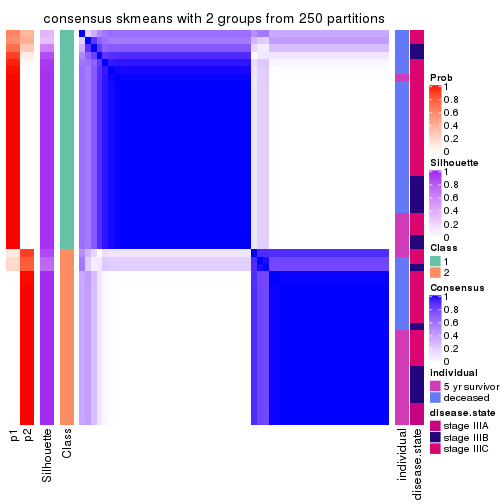
consensus_heatmap(res, k = 3)
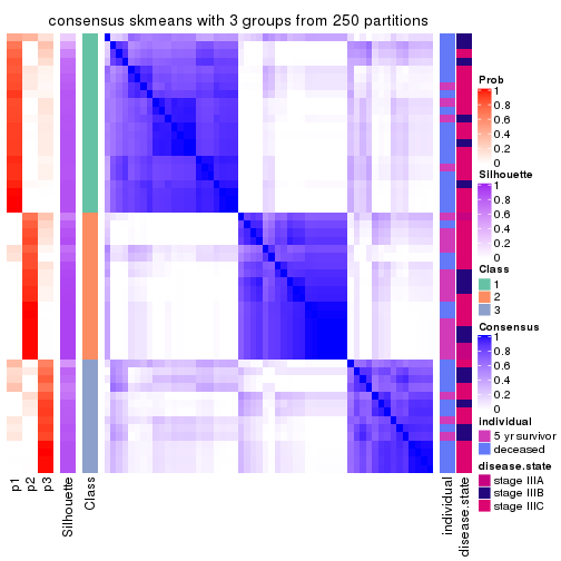
consensus_heatmap(res, k = 4)
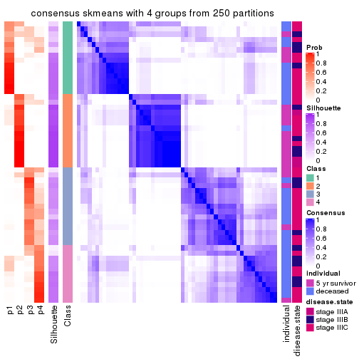
consensus_heatmap(res, k = 5)
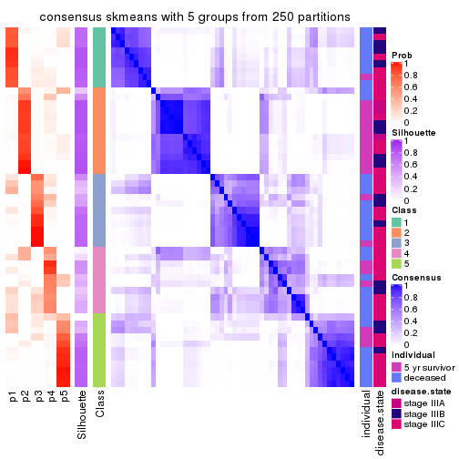
consensus_heatmap(res, k = 6)
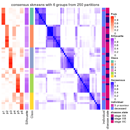
Heatmaps for the membership of samples in all partitions to see how consistent they are:
membership_heatmap(res, k = 2)

membership_heatmap(res, k = 3)
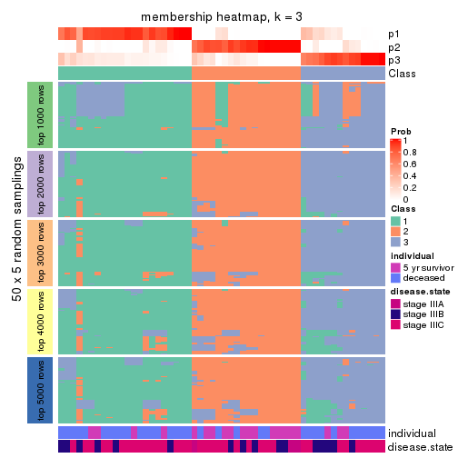
membership_heatmap(res, k = 4)
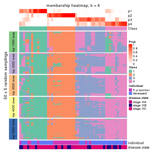
membership_heatmap(res, k = 5)
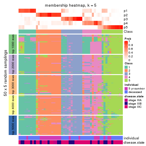
membership_heatmap(res, k = 6)
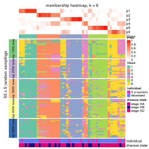
As soon as we have had the classes for columns, we can look for signatures which are significantly different between classes which can be candidate marks for certain classes. Following are the heatmaps for signatures.
Signature heatmaps where rows are scaled:
get_signatures(res, k = 2)
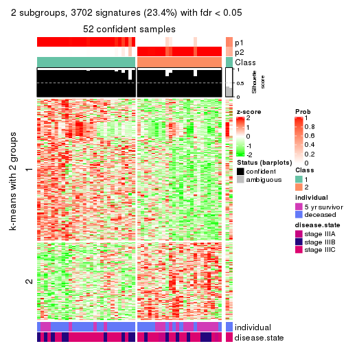
get_signatures(res, k = 3)
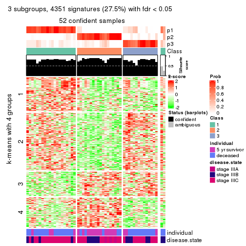
get_signatures(res, k = 4)
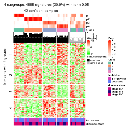
get_signatures(res, k = 5)
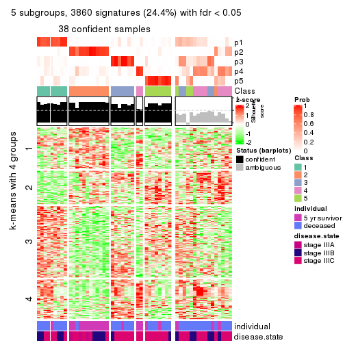
get_signatures(res, k = 6)
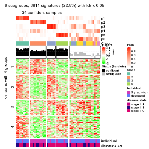
Signature heatmaps where rows are not scaled:
get_signatures(res, k = 2, scale_rows = FALSE)
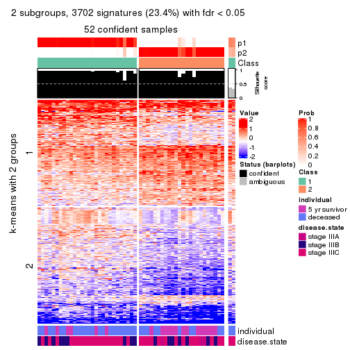
get_signatures(res, k = 3, scale_rows = FALSE)
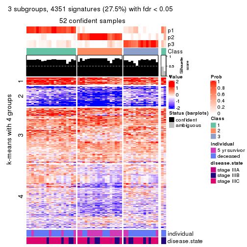
get_signatures(res, k = 4, scale_rows = FALSE)
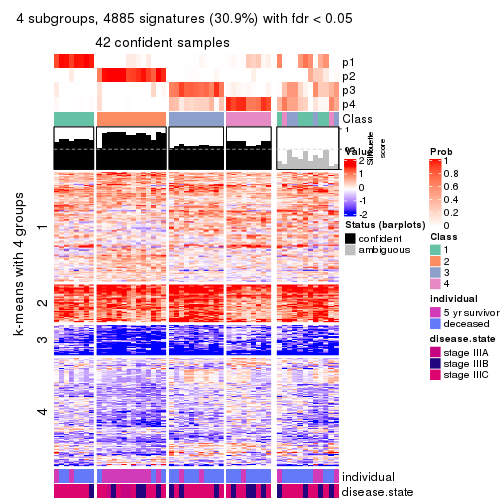
get_signatures(res, k = 5, scale_rows = FALSE)
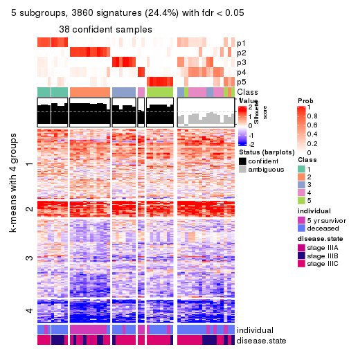
get_signatures(res, k = 6, scale_rows = FALSE)
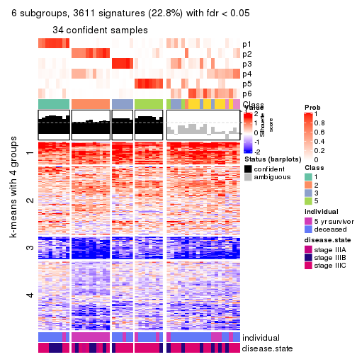
Compare the overlap of signatures from different k:
compare_signatures(res)
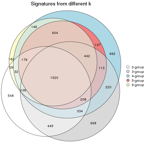
get_signature() returns a data frame invisibly. TO get the list of signatures, the function
call should be assigned to a variable explicitly. In following code, if plot argument is set
to FALSE, no heatmap is plotted while only the differential analysis is performed.
# code only for demonstration
tb = get_signature(res, k = ..., plot = FALSE)
An example of the output of tb is:
#>   which_row         fdr    mean_1    mean_2 scaled_mean_1 scaled_mean_2 km
#> 1        38 0.042760348  8.373488  9.131774    -0.5533452     0.5164555  1
#> 2        40 0.018707592  7.106213  8.469186    -0.6173731     0.5762149  1
#> 3        55 0.019134737 10.221463 11.207825    -0.6159697     0.5749050  1
#> 4        59 0.006059896  5.921854  7.869574    -0.6899429     0.6439467  1
#> 5        60 0.018055526  8.928898 10.211722    -0.6204761     0.5791110  1
#> 6        98 0.009384629 15.714769 14.887706     0.6635654    -0.6193277  2
...
The columns in tb are:
which_row: row indices corresponding to the input matrix.fdr: FDR for the differential test. mean_x: The mean value in group x.scaled_mean_x: The mean value in group x after rows are scaled.km: Row groups if k-means clustering is applied to rows.UMAP plot which shows how samples are separated.
dimension_reduction(res, k = 2, method = "UMAP")
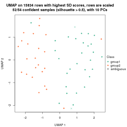
dimension_reduction(res, k = 3, method = "UMAP")
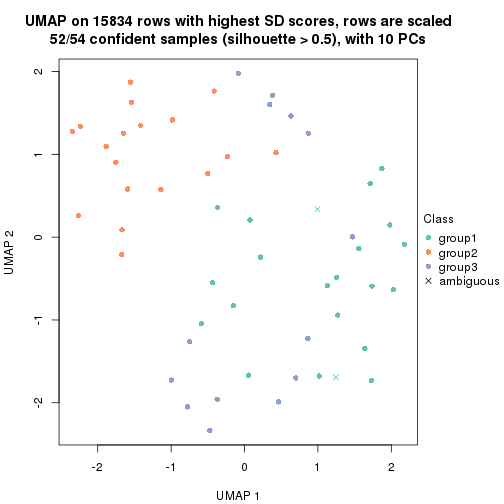
dimension_reduction(res, k = 4, method = "UMAP")
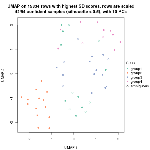
dimension_reduction(res, k = 5, method = "UMAP")
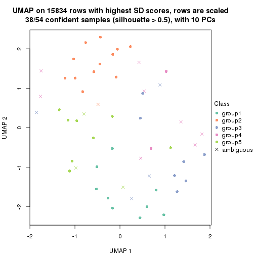
dimension_reduction(res, k = 6, method = "UMAP")
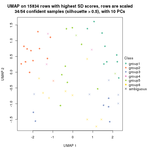
Following heatmap shows how subgroups are split when increasing k:
collect_classes(res)
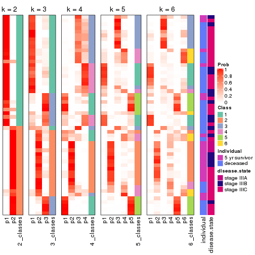
Test correlation between subgroups and known annotations. If the known annotation is numeric, one-way ANOVA test is applied, and if the known annotation is discrete, chi-squared contingency table test is applied.
test_to_known_factors(res)
#>             n individual(p) disease.state(p) k
#> SD:skmeans 52      0.014644           0.1555 2
#> SD:skmeans 52      0.001317           0.1210 3
#> SD:skmeans 42      0.001872           0.1812 4
#> SD:skmeans 38      0.000294           0.1559 5
#> SD:skmeans 34      0.000109           0.0958 6
If matrix rows can be associated to genes, consider to use functional_enrichment(res,
...) to perform function enrichment for the signature genes. See this vignette for more detailed explanations.
The object with results only for a single top-value method and a single partition method can be extracted as:
res = res_list["SD", "pam"]
# you can also extract it by
# res = res_list["SD:pam"]
A summary of res and all the functions that can be applied to it:
res
#> A 'ConsensusPartition' object with k = 2, 3, 4, 5, 6.
#>   On a matrix with 15834 rows and 54 columns.
#>   Top rows (1000, 2000, 3000, 4000, 5000) are extracted by 'SD' method.
#>   Subgroups are detected by 'pam' method.
#>   Performed in total 1250 partitions by row resampling.
#>   Best k for subgroups seems to be 2.
#>
#> Following methods can be applied to this 'ConsensusPartition' object:
#>  [1] "cola_report"             "collect_classes"         "collect_plots"
#>  [4] "collect_stats"           "colnames"                "compare_signatures"
#>  [7] "consensus_heatmap"       "dimension_reduction"     "functional_enrichment"
#> [10] "get_anno_col"            "get_anno"                "get_classes"
#> [13] "get_consensus"           "get_matrix"              "get_membership"
#> [16] "get_param"               "get_signatures"          "get_stats"
#> [19] "is_best_k"               "is_stable_k"             "membership_heatmap"
#> [22] "ncol"                    "nrow"                    "plot_ecdf"
#> [25] "rownames"                "select_partition_number" "show"
#> [28] "suggest_best_k"          "test_to_known_factors"
collect_plots() function collects all the plots made from res for all k (number of partitions)
into one single page to provide an easy and fast comparison between different k.
collect_plots(res)
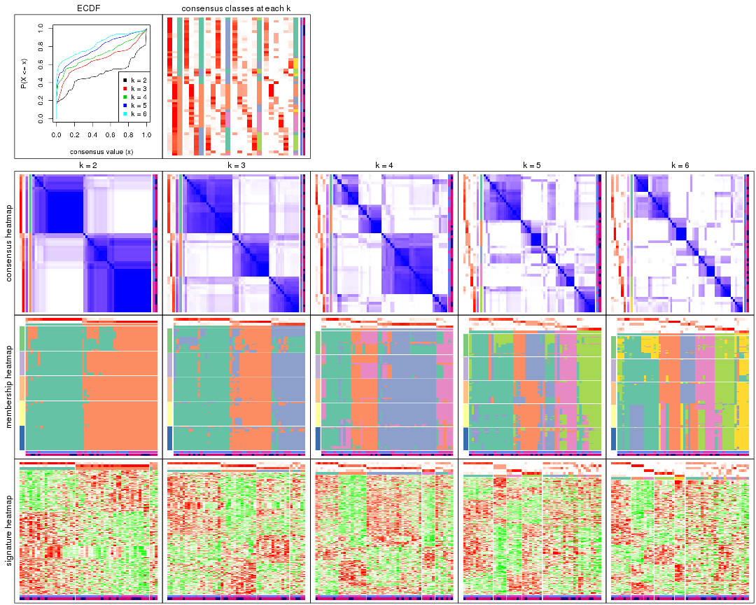
The plots are:
k and the heatmap of
predicted classes for each k.k.k.k.All the plots in panels can be made by individual functions and they are plotted later in this section.
select_partition_number() produces several plots showing different
statistics for choosing “optimized” k. There are following statistics:
k;k, the area increased is defined as \(A_k - A_{k-1}\).The detailed explanations of these statistics can be found in the cola vignette.
Generally speaking, lower PAC score, higher mean silhouette score or higher
concordance corresponds to better partition. Rand index and Jaccard index
measure how similar the current partition is compared to partition with k-1.
If they are too similar, we won't accept k is better than k-1.
select_partition_number(res)
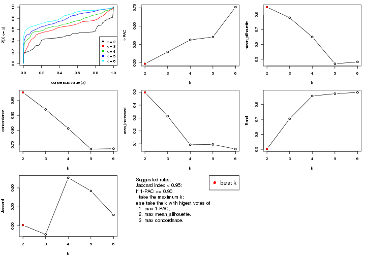
The numeric values for all these statistics can be obtained by get_stats().
get_stats(res)
#>   k 1-PAC mean_silhouette concordance area_increased  Rand Jaccard
#> 2 2 0.547           0.853       0.928         0.4982 0.502   0.502
#> 3 3 0.580           0.781       0.870         0.3148 0.704   0.477
#> 4 4 0.613           0.651       0.806         0.0931 0.856   0.627
#> 5 5 0.620           0.470       0.736         0.0952 0.871   0.592
#> 6 6 0.702           0.482       0.737         0.0593 0.880   0.529
suggest_best_k() suggests the best \(k\) based on these statistics. The rules are as follows:
suggest_best_k(res)
#> [1] 2
Following shows the table of the partitions (You need to click the show/hide
code output link to see it). The membership matrix (columns with name p*)
is inferred by
clue::cl_consensus()
function with the SE method. Basically the value in the membership matrix
represents the probability to belong to a certain group. The finall class
label for an item is determined with the group with highest probability it
belongs to.
In get_classes() function, the entropy is calculated from the membership
matrix and the silhouette score is calculated from the consensus matrix.
cbind(get_classes(res, k = 2), get_membership(res, k = 2))
#>           class entropy silhouette    p1    p2
#> GSM311939     2  0.0000      0.903 0.000 1.000
#> GSM311963     2  0.0000      0.903 0.000 1.000
#> GSM311973     2  0.0000      0.903 0.000 1.000
#> GSM311940     2  0.0000      0.903 0.000 1.000
#> GSM311953     2  0.0000      0.903 0.000 1.000
#> GSM311974     2  0.0000      0.903 0.000 1.000
#> GSM311975     2  0.4939      0.862 0.108 0.892
#> GSM311977     2  0.0000      0.903 0.000 1.000
#> GSM311982     1  0.5519      0.817 0.872 0.128
#> GSM311990     2  0.2948      0.887 0.052 0.948
#> GSM311943     1  0.0000      0.940 1.000 0.000
#> GSM311944     1  0.9580      0.266 0.620 0.380
#> GSM311946     2  0.0000      0.903 0.000 1.000
#> GSM311956     2  0.0000      0.903 0.000 1.000
#> GSM311967     2  0.0000      0.903 0.000 1.000
#> GSM311968     2  0.0376      0.902 0.004 0.996
#> GSM311972     1  0.0000      0.940 1.000 0.000
#> GSM311980     2  0.0000      0.903 0.000 1.000
#> GSM311981     2  0.9977      0.272 0.472 0.528
#> GSM311988     2  0.0000      0.903 0.000 1.000
#> GSM311957     2  0.5519      0.852 0.128 0.872
#> GSM311960     2  0.6887      0.816 0.184 0.816
#> GSM311971     2  0.9954      0.149 0.460 0.540
#> GSM311976     1  0.0000      0.940 1.000 0.000
#> GSM311978     1  0.0000      0.940 1.000 0.000
#> GSM311979     1  0.0000      0.940 1.000 0.000
#> GSM311983     1  0.4815      0.861 0.896 0.104
#> GSM311986     2  0.0000      0.903 0.000 1.000
#> GSM311991     1  0.6801      0.792 0.820 0.180
#> GSM311938     2  0.3879      0.874 0.076 0.924
#> GSM311941     1  0.0000      0.940 1.000 0.000
#> GSM311942     2  0.7139      0.806 0.196 0.804
#> GSM311945     2  0.7674      0.778 0.224 0.776
#> GSM311947     2  0.4298      0.872 0.088 0.912
#> GSM311948     2  0.0000      0.903 0.000 1.000
#> GSM311949     1  0.0000      0.940 1.000 0.000
#> GSM311950     2  0.0000      0.903 0.000 1.000
#> GSM311951     2  0.7139      0.806 0.196 0.804
#> GSM311952     1  0.5519      0.845 0.872 0.128
#> GSM311954     1  0.0000      0.940 1.000 0.000
#> GSM311955     1  0.0000      0.940 1.000 0.000
#> GSM311958     1  0.0000      0.940 1.000 0.000
#> GSM311959     1  0.0000      0.940 1.000 0.000
#> GSM311961     2  0.6712      0.811 0.176 0.824
#> GSM311962     1  0.0000      0.940 1.000 0.000
#> GSM311964     1  0.0000      0.940 1.000 0.000
#> GSM311965     2  0.7219      0.802 0.200 0.800
#> GSM311966     1  0.0000      0.940 1.000 0.000
#> GSM311969     1  0.0000      0.940 1.000 0.000
#> GSM311970     2  0.0000      0.903 0.000 1.000
#> GSM311984     1  0.6973      0.776 0.812 0.188
#> GSM311985     1  0.0000      0.940 1.000 0.000
#> GSM311987     1  0.2423      0.913 0.960 0.040
#> GSM311989     2  0.7219      0.802 0.200 0.800
cbind(get_classes(res, k = 3), get_membership(res, k = 3))
#>           class entropy silhouette    p1    p2    p3
#> GSM311939     2  0.0592      0.855 0.000 0.988 0.012
#> GSM311963     2  0.0000      0.856 0.000 1.000 0.000
#> GSM311973     2  0.6267      0.248 0.000 0.548 0.452
#> GSM311940     2  0.0000      0.856 0.000 1.000 0.000
#> GSM311953     2  0.1643      0.849 0.000 0.956 0.044
#> GSM311974     2  0.4062      0.770 0.000 0.836 0.164
#> GSM311975     1  0.3888      0.833 0.888 0.048 0.064
#> GSM311977     2  0.0000      0.856 0.000 1.000 0.000
#> GSM311982     3  0.5835      0.644 0.340 0.000 0.660
#> GSM311990     3  0.4059      0.777 0.012 0.128 0.860
#> GSM311943     1  0.1163      0.878 0.972 0.000 0.028
#> GSM311944     3  0.3038      0.843 0.104 0.000 0.896
#> GSM311946     2  0.1643      0.849 0.000 0.956 0.044
#> GSM311956     2  0.1289      0.852 0.000 0.968 0.032
#> GSM311967     2  0.2625      0.821 0.000 0.916 0.084
#> GSM311968     3  0.2878      0.793 0.000 0.096 0.904
#> GSM311972     1  0.3482      0.848 0.872 0.000 0.128
#> GSM311980     2  0.6192      0.342 0.000 0.580 0.420
#> GSM311981     2  0.7271      0.426 0.040 0.608 0.352
#> GSM311988     2  0.0000      0.856 0.000 1.000 0.000
#> GSM311957     3  0.7920      0.482 0.360 0.068 0.572
#> GSM311960     3  0.3875      0.859 0.068 0.044 0.888
#> GSM311971     1  0.7656      0.366 0.572 0.376 0.052
#> GSM311976     1  0.2066      0.889 0.940 0.000 0.060
#> GSM311978     1  0.2066      0.889 0.940 0.000 0.060
#> GSM311979     1  0.3686      0.838 0.860 0.000 0.140
#> GSM311983     1  0.1905      0.866 0.956 0.028 0.016
#> GSM311986     2  0.7478      0.509 0.308 0.632 0.060
#> GSM311991     1  0.5085      0.831 0.836 0.072 0.092
#> GSM311938     2  0.3583      0.802 0.044 0.900 0.056
#> GSM311941     3  0.5254      0.675 0.264 0.000 0.736
#> GSM311942     3  0.3091      0.857 0.072 0.016 0.912
#> GSM311945     3  0.3856      0.859 0.072 0.040 0.888
#> GSM311947     3  0.3941      0.741 0.000 0.156 0.844
#> GSM311948     3  0.5117      0.770 0.060 0.108 0.832
#> GSM311949     1  0.2165      0.889 0.936 0.000 0.064
#> GSM311950     2  0.2066      0.832 0.000 0.940 0.060
#> GSM311951     3  0.3856      0.859 0.072 0.040 0.888
#> GSM311952     1  0.2229      0.865 0.944 0.044 0.012
#> GSM311954     1  0.2448      0.888 0.924 0.000 0.076
#> GSM311955     1  0.0747      0.881 0.984 0.000 0.016
#> GSM311958     1  0.2165      0.889 0.936 0.000 0.064
#> GSM311959     1  0.2448      0.888 0.924 0.000 0.076
#> GSM311961     1  0.3009      0.848 0.920 0.052 0.028
#> GSM311962     1  0.1964      0.890 0.944 0.000 0.056
#> GSM311964     1  0.6168      0.249 0.588 0.000 0.412
#> GSM311965     3  0.2939      0.856 0.072 0.012 0.916
#> GSM311966     1  0.2066      0.889 0.940 0.000 0.060
#> GSM311969     1  0.0747      0.881 0.984 0.000 0.016
#> GSM311970     2  0.0000      0.856 0.000 1.000 0.000
#> GSM311984     1  0.2031      0.864 0.952 0.032 0.016
#> GSM311985     1  0.3412      0.852 0.876 0.000 0.124
#> GSM311987     1  0.4945      0.845 0.840 0.056 0.104
#> GSM311989     3  0.3572      0.858 0.060 0.040 0.900
cbind(get_classes(res, k = 4), get_membership(res, k = 4))
#>           class entropy silhouette    p1    p2    p3    p4
#> GSM311939     2  0.4222      0.778 0.000 0.728 0.000 0.272
#> GSM311963     2  0.4164      0.783 0.000 0.736 0.000 0.264
#> GSM311973     4  0.4319      0.562 0.228 0.012 0.000 0.760
#> GSM311940     2  0.4164      0.783 0.000 0.736 0.000 0.264
#> GSM311953     4  0.4072      0.323 0.000 0.252 0.000 0.748
#> GSM311974     4  0.2131      0.685 0.032 0.036 0.000 0.932
#> GSM311975     3  0.5187      0.687 0.004 0.228 0.728 0.040
#> GSM311977     2  0.4164      0.783 0.000 0.736 0.000 0.264
#> GSM311982     1  0.5632      0.544 0.712 0.000 0.092 0.196
#> GSM311990     1  0.6918     -0.242 0.472 0.108 0.000 0.420
#> GSM311943     3  0.1854      0.841 0.020 0.008 0.948 0.024
#> GSM311944     1  0.0000      0.688 1.000 0.000 0.000 0.000
#> GSM311946     4  0.1474      0.646 0.000 0.052 0.000 0.948
#> GSM311956     4  0.1356      0.661 0.008 0.032 0.000 0.960
#> GSM311967     2  0.0336      0.693 0.008 0.992 0.000 0.000
#> GSM311968     1  0.5696     -0.261 0.496 0.024 0.000 0.480
#> GSM311972     3  0.3636      0.795 0.172 0.008 0.820 0.000
#> GSM311980     4  0.4228      0.551 0.232 0.008 0.000 0.760
#> GSM311981     2  0.4247      0.640 0.104 0.836 0.016 0.044
#> GSM311988     2  0.4164      0.783 0.000 0.736 0.000 0.264
#> GSM311957     1  0.5435      0.149 0.564 0.000 0.420 0.016
#> GSM311960     1  0.3610      0.599 0.800 0.000 0.000 0.200
#> GSM311971     3  0.6134      0.671 0.084 0.008 0.676 0.232
#> GSM311976     3  0.2528      0.855 0.080 0.008 0.908 0.004
#> GSM311978     3  0.2149      0.854 0.088 0.000 0.912 0.000
#> GSM311979     3  0.5039      0.412 0.404 0.000 0.592 0.004
#> GSM311983     3  0.0707      0.844 0.000 0.000 0.980 0.020
#> GSM311986     3  0.6368      0.559 0.008 0.092 0.652 0.248
#> GSM311991     3  0.4677      0.664 0.000 0.316 0.680 0.004
#> GSM311938     2  0.6671      0.696 0.076 0.636 0.024 0.264
#> GSM311941     3  0.5754      0.366 0.428 0.016 0.548 0.008
#> GSM311942     1  0.1151      0.683 0.968 0.024 0.000 0.008
#> GSM311945     1  0.3494      0.623 0.824 0.000 0.004 0.172
#> GSM311947     2  0.3933      0.519 0.200 0.792 0.000 0.008
#> GSM311948     4  0.5332      0.146 0.480 0.004 0.004 0.512
#> GSM311949     3  0.2412      0.855 0.084 0.000 0.908 0.008
#> GSM311950     2  0.1042      0.700 0.008 0.972 0.000 0.020
#> GSM311951     1  0.0336      0.689 0.992 0.000 0.000 0.008
#> GSM311952     3  0.0921      0.844 0.000 0.000 0.972 0.028
#> GSM311954     3  0.3313      0.853 0.084 0.028 0.880 0.008
#> GSM311955     3  0.1745      0.843 0.008 0.020 0.952 0.020
#> GSM311958     3  0.2673      0.856 0.080 0.008 0.904 0.008
#> GSM311959     3  0.3105      0.854 0.084 0.020 0.888 0.008
#> GSM311961     3  0.0469      0.845 0.000 0.000 0.988 0.012
#> GSM311962     3  0.2198      0.856 0.072 0.008 0.920 0.000
#> GSM311964     1  0.4313      0.510 0.736 0.000 0.260 0.004
#> GSM311965     1  0.1042      0.685 0.972 0.020 0.000 0.008
#> GSM311966     3  0.2271      0.854 0.076 0.008 0.916 0.000
#> GSM311969     3  0.1749      0.841 0.012 0.012 0.952 0.024
#> GSM311970     2  0.4999      0.507 0.000 0.508 0.000 0.492
#> GSM311984     3  0.0469      0.845 0.000 0.000 0.988 0.012
#> GSM311985     3  0.3142      0.832 0.132 0.008 0.860 0.000
#> GSM311987     3  0.4274      0.839 0.096 0.064 0.832 0.008
#> GSM311989     1  0.0592      0.688 0.984 0.000 0.000 0.016
cbind(get_classes(res, k = 5), get_membership(res, k = 5))
#>           class entropy silhouette    p1    p2    p3    p4    p5
#> GSM311939     2  0.4906     0.5417 0.000 0.496 0.480 0.024 0.000
#> GSM311963     2  0.4829     0.5450 0.000 0.500 0.480 0.020 0.000
#> GSM311973     4  0.0510     0.7317 0.000 0.000 0.000 0.984 0.016
#> GSM311940     2  0.4829     0.5450 0.000 0.500 0.480 0.020 0.000
#> GSM311953     4  0.4854     0.4003 0.000 0.308 0.044 0.648 0.000
#> GSM311974     4  0.0451     0.7319 0.000 0.004 0.000 0.988 0.008
#> GSM311975     2  0.5731     0.0836 0.256 0.636 0.096 0.008 0.004
#> GSM311977     2  0.4829     0.5450 0.000 0.500 0.480 0.020 0.000
#> GSM311982     5  0.5470     0.6272 0.160 0.000 0.008 0.152 0.680
#> GSM311990     4  0.6555     0.4791 0.000 0.028 0.120 0.532 0.320
#> GSM311943     1  0.6005     0.4358 0.680 0.036 0.128 0.008 0.148
#> GSM311944     5  0.1220     0.7466 0.004 0.020 0.008 0.004 0.964
#> GSM311946     4  0.4555     0.1038 0.000 0.008 0.472 0.520 0.000
#> GSM311956     4  0.0579     0.7301 0.000 0.008 0.000 0.984 0.008
#> GSM311967     2  0.1216     0.4864 0.000 0.960 0.020 0.000 0.020
#> GSM311968     4  0.4151     0.5604 0.000 0.004 0.000 0.652 0.344
#> GSM311972     1  0.2890     0.6620 0.836 0.000 0.004 0.000 0.160
#> GSM311980     4  0.0290     0.7316 0.000 0.000 0.000 0.992 0.008
#> GSM311981     2  0.4442     0.2577 0.004 0.676 0.304 0.016 0.000
#> GSM311988     2  0.4829     0.5450 0.000 0.500 0.480 0.020 0.000
#> GSM311957     5  0.5618    -0.1019 0.472 0.020 0.016 0.012 0.480
#> GSM311960     5  0.3480     0.6302 0.000 0.000 0.000 0.248 0.752
#> GSM311971     1  0.4695     0.0876 0.524 0.004 0.464 0.000 0.008
#> GSM311976     1  0.2011     0.7103 0.908 0.004 0.000 0.000 0.088
#> GSM311978     1  0.2130     0.7108 0.908 0.000 0.012 0.000 0.080
#> GSM311979     1  0.4718     0.0763 0.540 0.000 0.016 0.000 0.444
#> GSM311983     1  0.2282     0.6737 0.920 0.036 0.032 0.008 0.004
#> GSM311986     3  0.3095     0.1133 0.096 0.004 0.868 0.008 0.024
#> GSM311991     1  0.4735     0.2316 0.524 0.460 0.016 0.000 0.000
#> GSM311938     3  0.4869    -0.4498 0.004 0.308 0.656 0.028 0.004
#> GSM311941     3  0.6749     0.2099 0.272 0.000 0.400 0.000 0.328
#> GSM311942     5  0.0566     0.7484 0.000 0.004 0.000 0.012 0.984
#> GSM311945     5  0.3282     0.6809 0.008 0.000 0.000 0.188 0.804
#> GSM311947     2  0.3003     0.3913 0.000 0.812 0.000 0.000 0.188
#> GSM311948     4  0.3835     0.6320 0.000 0.000 0.008 0.732 0.260
#> GSM311949     1  0.2408     0.7077 0.892 0.000 0.016 0.000 0.092
#> GSM311950     2  0.1405     0.4953 0.000 0.956 0.008 0.016 0.020
#> GSM311951     5  0.0404     0.7491 0.000 0.000 0.000 0.012 0.988
#> GSM311952     1  0.3345     0.6344 0.860 0.036 0.088 0.012 0.004
#> GSM311954     3  0.5825     0.1526 0.428 0.000 0.488 0.004 0.080
#> GSM311955     1  0.4880     0.4142 0.692 0.036 0.260 0.008 0.004
#> GSM311958     1  0.4362     0.6793 0.804 0.040 0.076 0.000 0.080
#> GSM311959     3  0.6027     0.1643 0.420 0.004 0.476 0.000 0.100
#> GSM311961     1  0.2177     0.6599 0.908 0.004 0.080 0.008 0.000
#> GSM311962     1  0.1831     0.7110 0.920 0.000 0.004 0.000 0.076
#> GSM311964     5  0.4537     0.2907 0.396 0.000 0.012 0.000 0.592
#> GSM311965     5  0.0566     0.7484 0.000 0.004 0.000 0.012 0.984
#> GSM311966     1  0.2172     0.7105 0.908 0.000 0.016 0.000 0.076
#> GSM311969     1  0.4928     0.3910 0.684 0.036 0.268 0.008 0.004
#> GSM311970     3  0.6483    -0.3302 0.000 0.192 0.452 0.356 0.000
#> GSM311984     1  0.1012     0.6902 0.968 0.000 0.020 0.012 0.000
#> GSM311985     1  0.2727     0.6954 0.868 0.000 0.016 0.000 0.116
#> GSM311987     3  0.6812     0.2297 0.344 0.044 0.500 0.000 0.112
#> GSM311989     5  0.1041     0.7474 0.000 0.004 0.000 0.032 0.964
cbind(get_classes(res, k = 6), get_membership(res, k = 6))
#>           class entropy silhouette    p1    p2    p3    p4    p5    p6
#> GSM311939     2  0.0000     0.6631 0.000 1.000 0.000 0.000 0.000 0.000
#> GSM311963     2  0.0000     0.6631 0.000 1.000 0.000 0.000 0.000 0.000
#> GSM311973     4  0.0458     0.6804 0.000 0.000 0.000 0.984 0.016 0.000
#> GSM311940     2  0.0000     0.6631 0.000 1.000 0.000 0.000 0.000 0.000
#> GSM311953     4  0.3789     0.2886 0.000 0.416 0.000 0.584 0.000 0.000
#> GSM311974     4  0.0363     0.6824 0.000 0.000 0.000 0.988 0.012 0.000
#> GSM311975     3  0.0458     0.3387 0.016 0.000 0.984 0.000 0.000 0.000
#> GSM311977     2  0.0000     0.6631 0.000 1.000 0.000 0.000 0.000 0.000
#> GSM311982     5  0.5198     0.5573 0.200 0.000 0.012 0.140 0.648 0.000
#> GSM311990     4  0.5551     0.4048 0.000 0.016 0.020 0.488 0.432 0.044
#> GSM311943     1  0.5059     0.4181 0.528 0.000 0.420 0.008 0.028 0.016
#> GSM311944     5  0.0713     0.7528 0.000 0.000 0.028 0.000 0.972 0.000
#> GSM311946     2  0.3823     0.3508 0.000 0.564 0.000 0.436 0.000 0.000
#> GSM311956     4  0.0363     0.6824 0.000 0.000 0.000 0.988 0.012 0.000
#> GSM311967     3  0.3950     0.4805 0.000 0.432 0.564 0.000 0.000 0.004
#> GSM311968     4  0.3998     0.3588 0.000 0.000 0.000 0.504 0.492 0.004
#> GSM311972     1  0.3436     0.5101 0.812 0.000 0.000 0.004 0.056 0.128
#> GSM311980     4  0.0363     0.6824 0.000 0.000 0.000 0.988 0.012 0.000
#> GSM311981     3  0.4269     0.1860 0.000 0.020 0.568 0.000 0.000 0.412
#> GSM311988     2  0.0000     0.6631 0.000 1.000 0.000 0.000 0.000 0.000
#> GSM311957     1  0.7240     0.2449 0.324 0.000 0.316 0.000 0.272 0.088
#> GSM311960     5  0.3804     0.5385 0.000 0.000 0.008 0.336 0.656 0.000
#> GSM311971     2  0.5238     0.2005 0.432 0.492 0.004 0.000 0.004 0.068
#> GSM311976     1  0.2773     0.5141 0.828 0.000 0.000 0.004 0.004 0.164
#> GSM311978     1  0.3087     0.5136 0.820 0.000 0.004 0.004 0.012 0.160
#> GSM311979     1  0.5697     0.2802 0.576 0.000 0.008 0.004 0.248 0.164
#> GSM311983     1  0.4440     0.4274 0.556 0.000 0.420 0.008 0.000 0.016
#> GSM311986     6  0.7362     0.1855 0.112 0.264 0.196 0.008 0.000 0.420
#> GSM311991     3  0.3944     0.2551 0.428 0.000 0.568 0.000 0.000 0.004
#> GSM311938     2  0.3864     0.0442 0.000 0.520 0.000 0.000 0.000 0.480
#> GSM311941     6  0.3313     0.5597 0.036 0.000 0.000 0.004 0.148 0.812
#> GSM311942     5  0.0146     0.7637 0.000 0.000 0.000 0.000 0.996 0.004
#> GSM311945     5  0.4062     0.5492 0.004 0.000 0.008 0.332 0.652 0.004
#> GSM311947     3  0.5601     0.5060 0.000 0.244 0.564 0.000 0.188 0.004
#> GSM311948     4  0.3899     0.4901 0.000 0.004 0.000 0.592 0.404 0.000
#> GSM311949     6  0.4128    -0.0153 0.488 0.000 0.000 0.004 0.004 0.504
#> GSM311950     3  0.3971     0.4653 0.000 0.448 0.548 0.000 0.000 0.004
#> GSM311951     5  0.0000     0.7649 0.000 0.000 0.000 0.000 1.000 0.000
#> GSM311952     1  0.4440     0.4274 0.556 0.000 0.420 0.008 0.000 0.016
#> GSM311954     6  0.2278     0.6738 0.128 0.004 0.000 0.000 0.000 0.868
#> GSM311955     1  0.4158     0.4278 0.572 0.000 0.416 0.004 0.000 0.008
#> GSM311958     1  0.5671     0.3941 0.460 0.000 0.416 0.004 0.004 0.116
#> GSM311959     6  0.2092     0.6753 0.124 0.000 0.000 0.000 0.000 0.876
#> GSM311961     1  0.0622     0.5409 0.980 0.000 0.000 0.008 0.000 0.012
#> GSM311962     1  0.2092     0.5225 0.876 0.000 0.000 0.000 0.000 0.124
#> GSM311964     1  0.5857    -0.1213 0.440 0.000 0.012 0.004 0.428 0.116
#> GSM311965     5  0.1765     0.7041 0.000 0.000 0.000 0.000 0.904 0.096
#> GSM311966     1  0.2092     0.5225 0.876 0.000 0.000 0.000 0.000 0.124
#> GSM311969     1  0.4656     0.4167 0.544 0.000 0.420 0.008 0.000 0.028
#> GSM311970     2  0.3765     0.4054 0.000 0.596 0.000 0.404 0.000 0.000
#> GSM311984     1  0.0665     0.5427 0.980 0.000 0.008 0.004 0.000 0.008
#> GSM311985     1  0.3018     0.5111 0.816 0.000 0.000 0.004 0.012 0.168
#> GSM311987     6  0.1643     0.6587 0.068 0.000 0.008 0.000 0.000 0.924
#> GSM311989     5  0.0260     0.7660 0.000 0.000 0.008 0.000 0.992 0.000
Heatmaps for the consensus matrix. It visualizes the probability of two samples to be in a same group.
consensus_heatmap(res, k = 2)
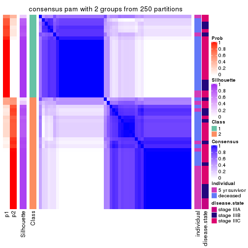
consensus_heatmap(res, k = 3)
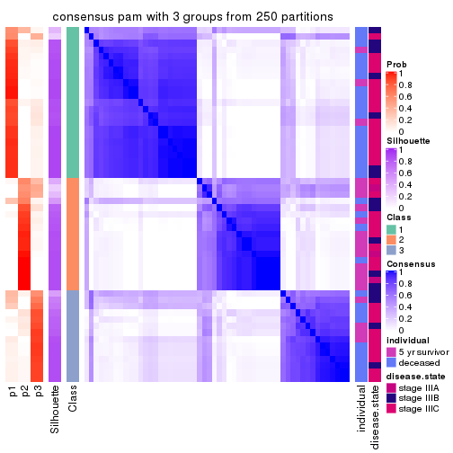
consensus_heatmap(res, k = 4)
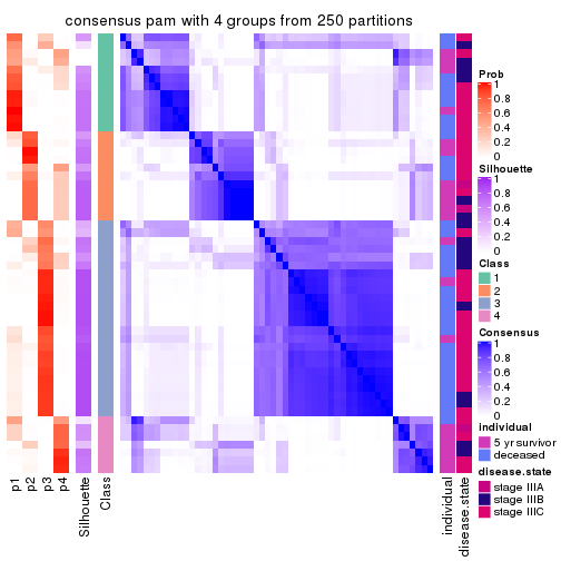
consensus_heatmap(res, k = 5)
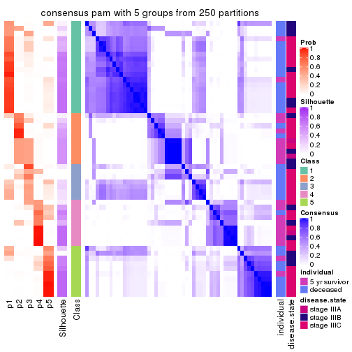
consensus_heatmap(res, k = 6)
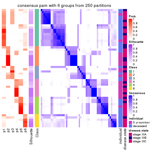
Heatmaps for the membership of samples in all partitions to see how consistent they are:
membership_heatmap(res, k = 2)

membership_heatmap(res, k = 3)
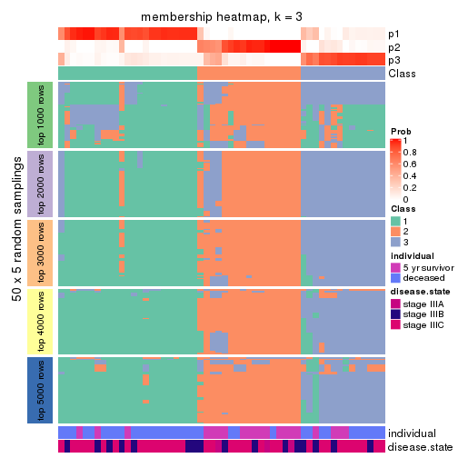
membership_heatmap(res, k = 4)
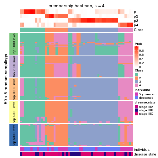
membership_heatmap(res, k = 5)
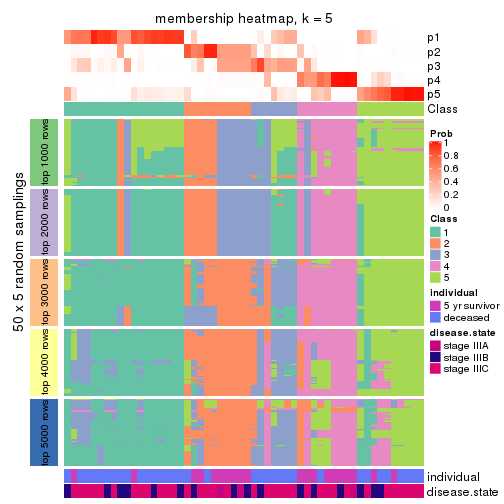
membership_heatmap(res, k = 6)
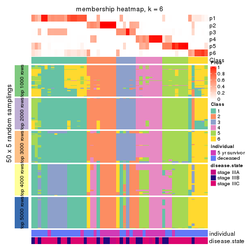
As soon as we have had the classes for columns, we can look for signatures which are significantly different between classes which can be candidate marks for certain classes. Following are the heatmaps for signatures.
Signature heatmaps where rows are scaled:
get_signatures(res, k = 2)
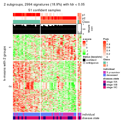
get_signatures(res, k = 3)
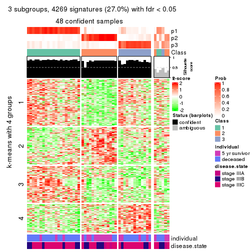
get_signatures(res, k = 4)
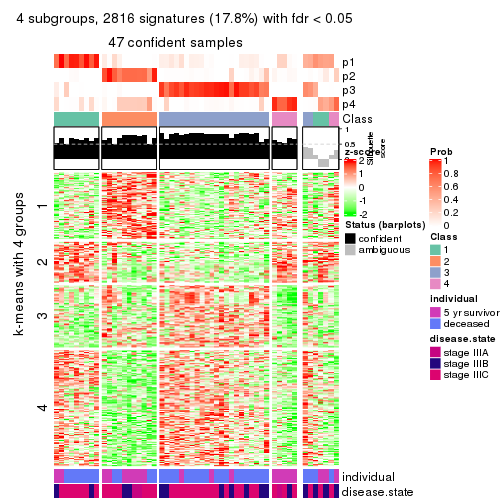
get_signatures(res, k = 5)
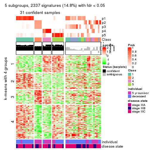
get_signatures(res, k = 6)
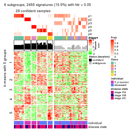
Signature heatmaps where rows are not scaled:
get_signatures(res, k = 2, scale_rows = FALSE)
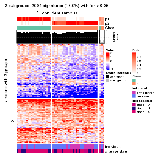
get_signatures(res, k = 3, scale_rows = FALSE)
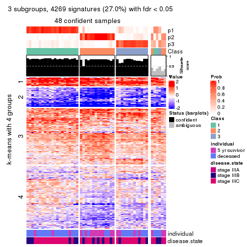
get_signatures(res, k = 4, scale_rows = FALSE)
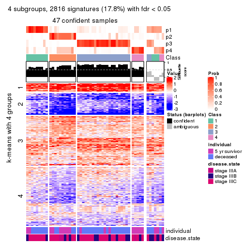
get_signatures(res, k = 5, scale_rows = FALSE)
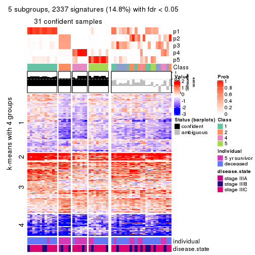
get_signatures(res, k = 6, scale_rows = FALSE)
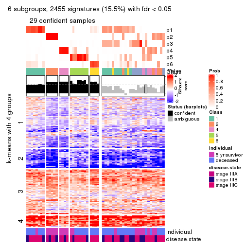
Compare the overlap of signatures from different k:
compare_signatures(res)
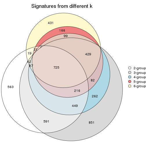
get_signature() returns a data frame invisibly. TO get the list of signatures, the function
call should be assigned to a variable explicitly. In following code, if plot argument is set
to FALSE, no heatmap is plotted while only the differential analysis is performed.
# code only for demonstration
tb = get_signature(res, k = ..., plot = FALSE)
An example of the output of tb is:
#>   which_row         fdr    mean_1    mean_2 scaled_mean_1 scaled_mean_2 km
#> 1        38 0.042760348  8.373488  9.131774    -0.5533452     0.5164555  1
#> 2        40 0.018707592  7.106213  8.469186    -0.6173731     0.5762149  1
#> 3        55 0.019134737 10.221463 11.207825    -0.6159697     0.5749050  1
#> 4        59 0.006059896  5.921854  7.869574    -0.6899429     0.6439467  1
#> 5        60 0.018055526  8.928898 10.211722    -0.6204761     0.5791110  1
#> 6        98 0.009384629 15.714769 14.887706     0.6635654    -0.6193277  2
...
The columns in tb are:
which_row: row indices corresponding to the input matrix.fdr: FDR for the differential test. mean_x: The mean value in group x.scaled_mean_x: The mean value in group x after rows are scaled.km: Row groups if k-means clustering is applied to rows.UMAP plot which shows how samples are separated.
dimension_reduction(res, k = 2, method = "UMAP")
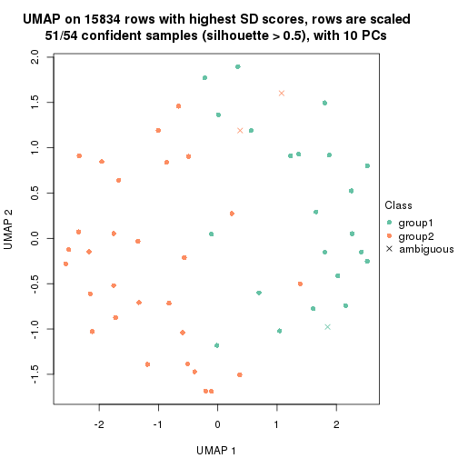
dimension_reduction(res, k = 3, method = "UMAP")
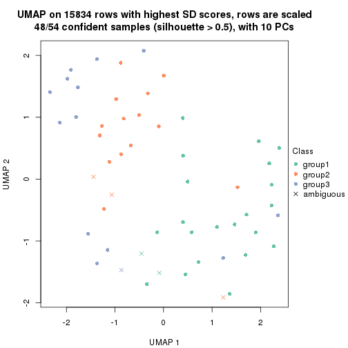
dimension_reduction(res, k = 4, method = "UMAP")
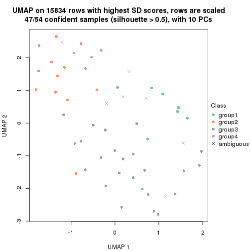
dimension_reduction(res, k = 5, method = "UMAP")
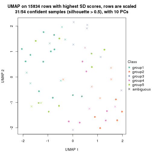
dimension_reduction(res, k = 6, method = "UMAP")
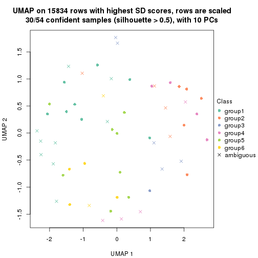
Following heatmap shows how subgroups are split when increasing k:
collect_classes(res)
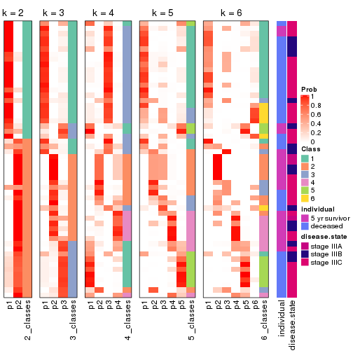
Test correlation between subgroups and known annotations. If the known annotation is numeric, one-way ANOVA test is applied, and if the known annotation is discrete, chi-squared contingency table test is applied.
test_to_known_factors(res)
#>         n individual(p) disease.state(p) k
#> SD:pam 51      0.011631            0.257 2
#> SD:pam 48      0.002288            0.192 3
#> SD:pam 47      0.000437            0.349 4
#> SD:pam 31      0.000519            0.149 5
#> SD:pam 30      0.001195            0.279 6
If matrix rows can be associated to genes, consider to use functional_enrichment(res,
...) to perform function enrichment for the signature genes. See this vignette for more detailed explanations.
The object with results only for a single top-value method and a single partition method can be extracted as:
res = res_list["SD", "mclust"]
# you can also extract it by
# res = res_list["SD:mclust"]
A summary of res and all the functions that can be applied to it:
res
#> A 'ConsensusPartition' object with k = 2, 3, 4, 5, 6.
#>   On a matrix with 15834 rows and 54 columns.
#>   Top rows (1000, 2000, 3000, 4000, 5000) are extracted by 'SD' method.
#>   Subgroups are detected by 'mclust' method.
#>   Performed in total 1250 partitions by row resampling.
#>   Best k for subgroups seems to be 5.
#>
#> Following methods can be applied to this 'ConsensusPartition' object:
#>  [1] "cola_report"             "collect_classes"         "collect_plots"
#>  [4] "collect_stats"           "colnames"                "compare_signatures"
#>  [7] "consensus_heatmap"       "dimension_reduction"     "functional_enrichment"
#> [10] "get_anno_col"            "get_anno"                "get_classes"
#> [13] "get_consensus"           "get_matrix"              "get_membership"
#> [16] "get_param"               "get_signatures"          "get_stats"
#> [19] "is_best_k"               "is_stable_k"             "membership_heatmap"
#> [22] "ncol"                    "nrow"                    "plot_ecdf"
#> [25] "rownames"                "select_partition_number" "show"
#> [28] "suggest_best_k"          "test_to_known_factors"
collect_plots() function collects all the plots made from res for all k (number of partitions)
into one single page to provide an easy and fast comparison between different k.
collect_plots(res)
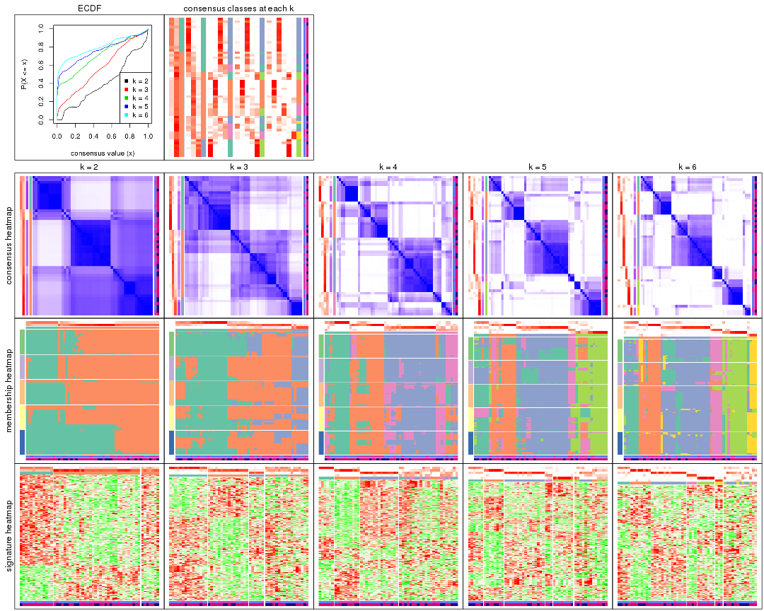
The plots are:
k and the heatmap of
predicted classes for each k.k.k.k.All the plots in panels can be made by individual functions and they are plotted later in this section.
select_partition_number() produces several plots showing different
statistics for choosing “optimized” k. There are following statistics:
k;k, the area increased is defined as \(A_k - A_{k-1}\).The detailed explanations of these statistics can be found in the cola vignette.
Generally speaking, lower PAC score, higher mean silhouette score or higher
concordance corresponds to better partition. Rand index and Jaccard index
measure how similar the current partition is compared to partition with k-1.
If they are too similar, we won't accept k is better than k-1.
select_partition_number(res)
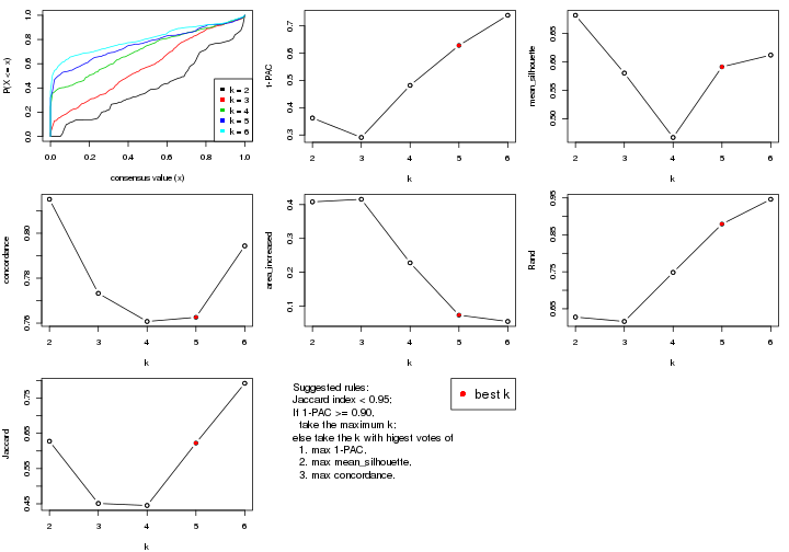
The numeric values for all these statistics can be obtained by get_stats().
get_stats(res)
#>   k 1-PAC mean_silhouette concordance area_increased  Rand Jaccard
#> 2 2 0.362           0.682       0.815         0.4080 0.628   0.628
#> 3 3 0.291           0.580       0.773         0.4157 0.616   0.451
#> 4 4 0.482           0.467       0.761         0.2279 0.748   0.445
#> 5 5 0.628           0.591       0.763         0.0733 0.879   0.622
#> 6 6 0.739           0.612       0.794         0.0546 0.946   0.792
suggest_best_k() suggests the best \(k\) based on these statistics. The rules are as follows:
suggest_best_k(res)
#> [1] 5
Following shows the table of the partitions (You need to click the show/hide
code output link to see it). The membership matrix (columns with name p*)
is inferred by
clue::cl_consensus()
function with the SE method. Basically the value in the membership matrix
represents the probability to belong to a certain group. The finall class
label for an item is determined with the group with highest probability it
belongs to.
In get_classes() function, the entropy is calculated from the membership
matrix and the silhouette score is calculated from the consensus matrix.
cbind(get_classes(res, k = 2), get_membership(res, k = 2))
#>           class entropy silhouette    p1    p2
#> GSM311939     2  0.8144     0.7450 0.252 0.748
#> GSM311963     2  0.8016     0.7488 0.244 0.756
#> GSM311973     2  0.6801     0.7565 0.180 0.820
#> GSM311940     2  0.8207     0.7422 0.256 0.744
#> GSM311953     2  0.8081     0.7467 0.248 0.752
#> GSM311974     2  0.7883     0.7501 0.236 0.764
#> GSM311975     2  0.9522    -0.2312 0.372 0.628
#> GSM311977     2  0.8144     0.7450 0.252 0.748
#> GSM311982     2  0.0376     0.7271 0.004 0.996
#> GSM311990     2  0.7815     0.7515 0.232 0.768
#> GSM311943     1  0.8909     0.9462 0.692 0.308
#> GSM311944     2  0.0376     0.7271 0.004 0.996
#> GSM311946     2  0.7528     0.7547 0.216 0.784
#> GSM311956     2  0.7883     0.7501 0.236 0.764
#> GSM311967     2  0.7950     0.7507 0.240 0.760
#> GSM311968     2  0.2948     0.7207 0.052 0.948
#> GSM311972     1  0.9286     0.9074 0.656 0.344
#> GSM311980     2  0.7883     0.7501 0.236 0.764
#> GSM311981     2  0.0672     0.7256 0.008 0.992
#> GSM311988     2  0.8207     0.7422 0.256 0.744
#> GSM311957     2  0.0376     0.7271 0.004 0.996
#> GSM311960     2  0.0376     0.7295 0.004 0.996
#> GSM311971     2  0.0376     0.7280 0.004 0.996
#> GSM311976     2  0.7139     0.4397 0.196 0.804
#> GSM311978     2  0.9635    -0.2643 0.388 0.612
#> GSM311979     2  0.0376     0.7271 0.004 0.996
#> GSM311983     1  0.8813     0.9428 0.700 0.300
#> GSM311986     2  0.4939     0.6159 0.108 0.892
#> GSM311991     2  0.7299     0.4083 0.204 0.796
#> GSM311938     2  0.7950     0.7522 0.240 0.760
#> GSM311941     1  0.9977     0.6923 0.528 0.472
#> GSM311942     2  0.2948     0.7207 0.052 0.948
#> GSM311945     2  0.1633     0.7267 0.024 0.976
#> GSM311947     2  0.7815     0.7515 0.232 0.768
#> GSM311948     2  0.6801     0.7564 0.180 0.820
#> GSM311949     2  0.7056     0.4607 0.192 0.808
#> GSM311950     2  0.8144     0.7443 0.252 0.748
#> GSM311951     2  0.2948     0.7207 0.052 0.948
#> GSM311952     1  0.8909     0.9462 0.692 0.308
#> GSM311954     2  0.8909     0.0687 0.308 0.692
#> GSM311955     1  0.8909     0.9462 0.692 0.308
#> GSM311958     1  0.8909     0.9462 0.692 0.308
#> GSM311959     2  1.0000    -0.6311 0.496 0.504
#> GSM311961     1  0.8813     0.9428 0.700 0.300
#> GSM311962     1  0.8813     0.9428 0.700 0.300
#> GSM311964     2  0.3431     0.6776 0.064 0.936
#> GSM311965     2  0.2778     0.7222 0.048 0.952
#> GSM311966     1  0.8813     0.9428 0.700 0.300
#> GSM311969     1  0.8909     0.9462 0.692 0.308
#> GSM311970     2  0.8016     0.7488 0.244 0.756
#> GSM311984     1  0.9996     0.6328 0.512 0.488
#> GSM311985     1  0.8909     0.9462 0.692 0.308
#> GSM311987     2  0.2778     0.7016 0.048 0.952
#> GSM311989     2  0.2948     0.7207 0.052 0.948
cbind(get_classes(res, k = 3), get_membership(res, k = 3))
#>           class entropy silhouette    p1    p2    p3
#> GSM311939     2  0.3695      0.592 0.012 0.880 0.108
#> GSM311963     2  0.3539      0.597 0.012 0.888 0.100
#> GSM311973     2  0.3983      0.600 0.004 0.852 0.144
#> GSM311940     2  0.4128      0.548 0.012 0.856 0.132
#> GSM311953     2  0.3715      0.611 0.004 0.868 0.128
#> GSM311974     2  0.3879      0.596 0.000 0.848 0.152
#> GSM311975     1  0.5803      0.614 0.736 0.248 0.016
#> GSM311977     2  0.3293      0.590 0.012 0.900 0.088
#> GSM311982     2  0.8825      0.347 0.336 0.532 0.132
#> GSM311990     2  0.5902      0.447 0.004 0.680 0.316
#> GSM311943     1  0.1919      0.770 0.956 0.024 0.020
#> GSM311944     2  0.9090      0.357 0.332 0.512 0.156
#> GSM311946     2  0.6306      0.572 0.052 0.748 0.200
#> GSM311956     2  0.3879      0.596 0.000 0.848 0.152
#> GSM311967     2  0.7148      0.553 0.108 0.716 0.176
#> GSM311968     3  0.4047      0.877 0.004 0.148 0.848
#> GSM311972     1  0.3193      0.750 0.896 0.100 0.004
#> GSM311980     2  0.3879      0.596 0.000 0.848 0.152
#> GSM311981     2  0.6912      0.396 0.344 0.628 0.028
#> GSM311988     2  0.4575      0.545 0.012 0.828 0.160
#> GSM311957     2  0.8373      0.238 0.388 0.524 0.088
#> GSM311960     3  0.6495      0.175 0.004 0.460 0.536
#> GSM311971     2  0.8436      0.516 0.224 0.616 0.160
#> GSM311976     1  0.6386      0.283 0.584 0.412 0.004
#> GSM311978     1  0.6180      0.460 0.660 0.332 0.008
#> GSM311979     2  0.7549      0.124 0.436 0.524 0.040
#> GSM311983     1  0.0000      0.769 1.000 0.000 0.000
#> GSM311986     2  0.6843      0.457 0.332 0.640 0.028
#> GSM311991     1  0.6647      0.383 0.592 0.396 0.012
#> GSM311938     2  0.6585      0.570 0.244 0.712 0.044
#> GSM311941     1  0.5734      0.681 0.788 0.164 0.048
#> GSM311942     3  0.4047      0.877 0.004 0.148 0.848
#> GSM311945     3  0.7333      0.695 0.116 0.180 0.704
#> GSM311947     2  0.5678      0.444 0.000 0.684 0.316
#> GSM311948     2  0.5902      0.443 0.004 0.680 0.316
#> GSM311949     1  0.6318      0.418 0.636 0.356 0.008
#> GSM311950     2  0.3551      0.548 0.000 0.868 0.132
#> GSM311951     3  0.4047      0.877 0.004 0.148 0.848
#> GSM311952     1  0.0829      0.768 0.984 0.004 0.012
#> GSM311954     1  0.6553      0.295 0.580 0.412 0.008
#> GSM311955     1  0.0848      0.770 0.984 0.008 0.008
#> GSM311958     1  0.0000      0.769 1.000 0.000 0.000
#> GSM311959     1  0.4953      0.691 0.808 0.176 0.016
#> GSM311961     1  0.0000      0.769 1.000 0.000 0.000
#> GSM311962     1  0.0000      0.769 1.000 0.000 0.000
#> GSM311964     1  0.7681      0.189 0.540 0.412 0.048
#> GSM311965     3  0.4047      0.877 0.004 0.148 0.848
#> GSM311966     1  0.0475      0.769 0.992 0.004 0.004
#> GSM311969     1  0.2743      0.765 0.928 0.052 0.020
#> GSM311970     2  0.1753      0.610 0.000 0.952 0.048
#> GSM311984     1  0.4228      0.714 0.844 0.148 0.008
#> GSM311985     1  0.0000      0.769 1.000 0.000 0.000
#> GSM311987     2  0.6603      0.435 0.332 0.648 0.020
#> GSM311989     3  0.4047      0.877 0.004 0.148 0.848
cbind(get_classes(res, k = 4), get_membership(res, k = 4))
#>           class entropy silhouette    p1    p2    p3    p4
#> GSM311939     2  0.0188     0.7114 0.000 0.996 0.004 0.000
#> GSM311963     2  0.0188     0.7104 0.000 0.996 0.000 0.004
#> GSM311973     2  0.5337     0.3088 0.424 0.564 0.000 0.012
#> GSM311940     2  0.0188     0.7114 0.000 0.996 0.004 0.000
#> GSM311953     2  0.2125     0.7032 0.076 0.920 0.000 0.004
#> GSM311974     2  0.4560     0.5317 0.296 0.700 0.000 0.004
#> GSM311975     3  0.2704     0.6248 0.000 0.000 0.876 0.124
#> GSM311977     2  0.0188     0.7114 0.000 0.996 0.004 0.000
#> GSM311982     1  0.5421     0.3016 0.548 0.004 0.008 0.440
#> GSM311990     4  0.7748    -0.1213 0.332 0.244 0.000 0.424
#> GSM311943     3  0.1004     0.7484 0.004 0.000 0.972 0.024
#> GSM311944     1  0.8600     0.0808 0.476 0.112 0.312 0.100
#> GSM311946     2  0.4381     0.6541 0.160 0.804 0.008 0.028
#> GSM311956     2  0.5097     0.3101 0.428 0.568 0.000 0.004
#> GSM311967     4  0.7784     0.1467 0.000 0.292 0.280 0.428
#> GSM311968     1  0.0000     0.7695 1.000 0.000 0.000 0.000
#> GSM311972     3  0.4624     0.4876 0.000 0.000 0.660 0.340
#> GSM311980     2  0.5137     0.2553 0.452 0.544 0.000 0.004
#> GSM311981     4  0.7469     0.2086 0.000 0.176 0.392 0.432
#> GSM311988     2  0.0188     0.7114 0.000 0.996 0.004 0.000
#> GSM311957     3  0.9109    -0.0783 0.180 0.092 0.384 0.344
#> GSM311960     1  0.4605     0.2671 0.664 0.336 0.000 0.000
#> GSM311971     4  0.8372     0.1841 0.044 0.292 0.184 0.480
#> GSM311976     3  0.7253     0.2391 0.000 0.172 0.520 0.308
#> GSM311978     4  0.5168    -0.2896 0.000 0.004 0.492 0.504
#> GSM311979     4  0.7319     0.0861 0.168 0.008 0.264 0.560
#> GSM311983     3  0.2345     0.7347 0.000 0.000 0.900 0.100
#> GSM311986     3  0.4204     0.4951 0.000 0.192 0.788 0.020
#> GSM311991     4  0.7119     0.0620 0.000 0.128 0.432 0.440
#> GSM311938     2  0.6750    -0.0354 0.000 0.540 0.356 0.104
#> GSM311941     3  0.1767     0.7220 0.012 0.000 0.944 0.044
#> GSM311942     1  0.0000     0.7695 1.000 0.000 0.000 0.000
#> GSM311945     1  0.0000     0.7695 1.000 0.000 0.000 0.000
#> GSM311947     4  0.7748    -0.1213 0.332 0.244 0.000 0.424
#> GSM311948     1  0.4585     0.2972 0.668 0.332 0.000 0.000
#> GSM311949     3  0.5165     0.2080 0.000 0.004 0.512 0.484
#> GSM311950     2  0.4188     0.5258 0.000 0.752 0.004 0.244
#> GSM311951     1  0.0000     0.7695 1.000 0.000 0.000 0.000
#> GSM311952     3  0.1474     0.7473 0.000 0.000 0.948 0.052
#> GSM311954     3  0.1510     0.7272 0.000 0.028 0.956 0.016
#> GSM311955     3  0.0000     0.7435 0.000 0.000 1.000 0.000
#> GSM311958     3  0.0921     0.7491 0.000 0.000 0.972 0.028
#> GSM311959     3  0.1389     0.7151 0.000 0.000 0.952 0.048
#> GSM311961     3  0.2216     0.7380 0.000 0.000 0.908 0.092
#> GSM311962     3  0.2408     0.7327 0.000 0.000 0.896 0.104
#> GSM311964     4  0.5783    -0.1459 0.024 0.004 0.412 0.560
#> GSM311965     1  0.0000     0.7695 1.000 0.000 0.000 0.000
#> GSM311966     3  0.4164     0.5885 0.000 0.000 0.736 0.264
#> GSM311969     3  0.0000     0.7435 0.000 0.000 1.000 0.000
#> GSM311970     2  0.3123     0.6111 0.000 0.844 0.000 0.156
#> GSM311984     3  0.0000     0.7435 0.000 0.000 1.000 0.000
#> GSM311985     3  0.2469     0.7303 0.000 0.000 0.892 0.108
#> GSM311987     3  0.7028     0.0898 0.000 0.228 0.576 0.196
#> GSM311989     1  0.0000     0.7695 1.000 0.000 0.000 0.000
cbind(get_classes(res, k = 5), get_membership(res, k = 5))
#>           class entropy silhouette    p1    p2    p3    p4    p5
#> GSM311939     2  0.0000     0.7341 0.000 1.000 0.000 0.000 0.000
#> GSM311963     2  0.0000     0.7341 0.000 1.000 0.000 0.000 0.000
#> GSM311973     5  0.8097     0.2009 0.104 0.272 0.000 0.248 0.376
#> GSM311940     2  0.0000     0.7341 0.000 1.000 0.000 0.000 0.000
#> GSM311953     2  0.3993     0.6167 0.028 0.756 0.000 0.216 0.000
#> GSM311974     2  0.8028    -0.0499 0.104 0.392 0.000 0.216 0.288
#> GSM311975     3  0.3690     0.6742 0.020 0.000 0.780 0.200 0.000
#> GSM311977     2  0.0000     0.7341 0.000 1.000 0.000 0.000 0.000
#> GSM311982     5  0.4649     0.1909 0.404 0.000 0.016 0.000 0.580
#> GSM311990     4  0.6355     0.7773 0.184 0.016 0.000 0.584 0.216
#> GSM311943     3  0.1043     0.7586 0.040 0.000 0.960 0.000 0.000
#> GSM311944     5  0.3231     0.4288 0.004 0.000 0.196 0.000 0.800
#> GSM311946     2  0.6204     0.5540 0.184 0.668 0.016 0.044 0.088
#> GSM311956     5  0.8081     0.1831 0.104 0.288 0.000 0.232 0.376
#> GSM311967     4  0.6713     0.5828 0.172 0.044 0.204 0.580 0.000
#> GSM311968     5  0.0510     0.6730 0.016 0.000 0.000 0.000 0.984
#> GSM311972     3  0.3561     0.3962 0.260 0.000 0.740 0.000 0.000
#> GSM311980     5  0.8037     0.2473 0.104 0.248 0.000 0.248 0.400
#> GSM311981     3  0.6004     0.3301 0.024 0.060 0.516 0.400 0.000
#> GSM311988     2  0.0000     0.7341 0.000 1.000 0.000 0.000 0.000
#> GSM311957     1  0.6813     0.6299 0.436 0.008 0.344 0.000 0.212
#> GSM311960     5  0.3596     0.5941 0.000 0.016 0.000 0.200 0.784
#> GSM311971     1  0.4899     0.6448 0.736 0.112 0.144 0.000 0.008
#> GSM311976     3  0.5376    -0.4746 0.424 0.056 0.520 0.000 0.000
#> GSM311978     1  0.3876     0.8167 0.684 0.000 0.316 0.000 0.000
#> GSM311979     1  0.4840     0.7993 0.688 0.000 0.248 0.000 0.064
#> GSM311983     3  0.0703     0.7643 0.024 0.000 0.976 0.000 0.000
#> GSM311986     3  0.4342     0.6235 0.012 0.016 0.724 0.248 0.000
#> GSM311991     3  0.6305     0.4931 0.060 0.060 0.580 0.300 0.000
#> GSM311938     2  0.7253     0.1432 0.060 0.480 0.312 0.148 0.000
#> GSM311941     3  0.1310     0.7550 0.020 0.000 0.956 0.000 0.024
#> GSM311942     5  0.0000     0.6746 0.000 0.000 0.000 0.000 1.000
#> GSM311945     5  0.0290     0.6728 0.000 0.000 0.008 0.000 0.992
#> GSM311947     4  0.6379     0.7757 0.184 0.016 0.000 0.580 0.220
#> GSM311948     5  0.5071     0.5648 0.092 0.128 0.016 0.012 0.752
#> GSM311949     1  0.4074     0.7753 0.636 0.000 0.364 0.000 0.000
#> GSM311950     2  0.5546     0.3703 0.176 0.648 0.000 0.176 0.000
#> GSM311951     5  0.0000     0.6746 0.000 0.000 0.000 0.000 1.000
#> GSM311952     3  0.1270     0.7524 0.052 0.000 0.948 0.000 0.000
#> GSM311954     3  0.3863     0.6845 0.020 0.012 0.792 0.176 0.000
#> GSM311955     3  0.0566     0.7652 0.012 0.000 0.984 0.004 0.000
#> GSM311958     3  0.1168     0.7650 0.032 0.000 0.960 0.008 0.000
#> GSM311959     3  0.3656     0.6770 0.020 0.000 0.784 0.196 0.000
#> GSM311961     3  0.1043     0.7594 0.040 0.000 0.960 0.000 0.000
#> GSM311962     3  0.0703     0.7646 0.024 0.000 0.976 0.000 0.000
#> GSM311964     1  0.4235     0.8087 0.656 0.000 0.336 0.000 0.008
#> GSM311965     5  0.0162     0.6744 0.000 0.000 0.004 0.000 0.996
#> GSM311966     3  0.1908     0.7090 0.092 0.000 0.908 0.000 0.000
#> GSM311969     3  0.0880     0.7619 0.032 0.000 0.968 0.000 0.000
#> GSM311970     2  0.3946     0.5890 0.080 0.800 0.000 0.120 0.000
#> GSM311984     3  0.0703     0.7649 0.024 0.000 0.976 0.000 0.000
#> GSM311985     3  0.1430     0.7624 0.052 0.000 0.944 0.004 0.000
#> GSM311987     3  0.5099     0.4901 0.020 0.016 0.596 0.368 0.000
#> GSM311989     5  0.0000     0.6746 0.000 0.000 0.000 0.000 1.000
cbind(get_classes(res, k = 6), get_membership(res, k = 6))
#>           class entropy silhouette    p1    p2    p3    p4    p5    p6
#> GSM311939     2  0.0260      0.824 0.000 0.992 0.000 0.000 0.000 0.008
#> GSM311963     2  0.0146      0.825 0.000 0.996 0.000 0.000 0.000 0.004
#> GSM311973     4  0.2499      0.870 0.000 0.048 0.000 0.880 0.072 0.000
#> GSM311940     2  0.0146      0.826 0.000 0.996 0.000 0.000 0.000 0.004
#> GSM311953     2  0.3265      0.556 0.004 0.748 0.000 0.248 0.000 0.000
#> GSM311974     4  0.2608      0.857 0.000 0.080 0.000 0.872 0.048 0.000
#> GSM311975     3  0.5091      0.522 0.224 0.000 0.652 0.112 0.000 0.012
#> GSM311977     2  0.0000      0.826 0.000 1.000 0.000 0.000 0.000 0.000
#> GSM311982     5  0.3872      0.378 0.392 0.000 0.004 0.000 0.604 0.000
#> GSM311990     6  0.1858      0.689 0.000 0.004 0.000 0.000 0.092 0.904
#> GSM311943     3  0.1410      0.697 0.044 0.000 0.944 0.004 0.000 0.008
#> GSM311944     5  0.0951      0.831 0.004 0.000 0.008 0.000 0.968 0.020
#> GSM311946     4  0.4676      0.344 0.040 0.384 0.000 0.572 0.004 0.000
#> GSM311956     4  0.2563      0.871 0.000 0.052 0.000 0.876 0.072 0.000
#> GSM311967     6  0.1894      0.670 0.016 0.012 0.040 0.004 0.000 0.928
#> GSM311968     5  0.1141      0.814 0.000 0.000 0.000 0.052 0.948 0.000
#> GSM311972     3  0.3765     -0.257 0.404 0.000 0.596 0.000 0.000 0.000
#> GSM311980     4  0.2457      0.859 0.000 0.036 0.000 0.880 0.084 0.000
#> GSM311981     3  0.6850      0.331 0.196 0.008 0.524 0.096 0.000 0.176
#> GSM311988     2  0.0000      0.826 0.000 1.000 0.000 0.000 0.000 0.000
#> GSM311957     1  0.6078      0.474 0.420 0.004 0.352 0.000 0.224 0.000
#> GSM311960     5  0.3881      0.301 0.000 0.004 0.000 0.396 0.600 0.000
#> GSM311971     1  0.4180      0.543 0.760 0.004 0.060 0.164 0.012 0.000
#> GSM311976     3  0.4408     -0.348 0.416 0.004 0.560 0.000 0.000 0.020
#> GSM311978     1  0.3371      0.731 0.708 0.000 0.292 0.000 0.000 0.000
#> GSM311979     1  0.3618      0.732 0.768 0.000 0.192 0.000 0.040 0.000
#> GSM311983     3  0.1492      0.694 0.036 0.000 0.940 0.000 0.000 0.024
#> GSM311986     3  0.6744      0.137 0.076 0.020 0.500 0.096 0.000 0.308
#> GSM311991     3  0.6154      0.475 0.228 0.004 0.588 0.104 0.000 0.076
#> GSM311938     2  0.6364      0.435 0.196 0.592 0.140 0.048 0.000 0.024
#> GSM311941     3  0.1675      0.686 0.008 0.000 0.936 0.000 0.032 0.024
#> GSM311942     5  0.0000      0.841 0.000 0.000 0.000 0.000 1.000 0.000
#> GSM311945     5  0.0146      0.841 0.004 0.000 0.000 0.000 0.996 0.000
#> GSM311947     6  0.1858      0.689 0.000 0.004 0.000 0.000 0.092 0.904
#> GSM311948     5  0.4412      0.379 0.012 0.024 0.000 0.320 0.644 0.000
#> GSM311949     1  0.3937      0.572 0.572 0.000 0.424 0.000 0.000 0.004
#> GSM311950     2  0.3607      0.562 0.000 0.652 0.000 0.000 0.000 0.348
#> GSM311951     5  0.0000      0.841 0.000 0.000 0.000 0.000 1.000 0.000
#> GSM311952     3  0.1141      0.693 0.052 0.000 0.948 0.000 0.000 0.000
#> GSM311954     3  0.5277      0.543 0.208 0.000 0.660 0.096 0.000 0.036
#> GSM311955     3  0.0632      0.703 0.024 0.000 0.976 0.000 0.000 0.000
#> GSM311958     3  0.1082      0.702 0.040 0.000 0.956 0.004 0.000 0.000
#> GSM311959     3  0.5184      0.533 0.212 0.000 0.656 0.112 0.000 0.020
#> GSM311961     3  0.1500      0.690 0.052 0.000 0.936 0.000 0.000 0.012
#> GSM311962     3  0.1176      0.698 0.020 0.000 0.956 0.000 0.000 0.024
#> GSM311964     1  0.4493      0.708 0.636 0.000 0.312 0.000 0.052 0.000
#> GSM311965     5  0.0146      0.841 0.004 0.000 0.000 0.000 0.996 0.000
#> GSM311966     3  0.3168      0.457 0.172 0.000 0.804 0.000 0.000 0.024
#> GSM311969     3  0.1552      0.701 0.036 0.000 0.940 0.004 0.000 0.020
#> GSM311970     2  0.2823      0.732 0.000 0.796 0.000 0.000 0.000 0.204
#> GSM311984     3  0.1616      0.693 0.048 0.000 0.932 0.000 0.000 0.020
#> GSM311985     3  0.1003      0.704 0.028 0.000 0.964 0.004 0.000 0.004
#> GSM311987     6  0.7456      0.074 0.224 0.004 0.300 0.116 0.000 0.356
#> GSM311989     5  0.0000      0.841 0.000 0.000 0.000 0.000 1.000 0.000
Heatmaps for the consensus matrix. It visualizes the probability of two samples to be in a same group.
consensus_heatmap(res, k = 2)
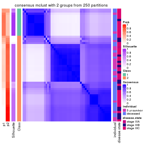
consensus_heatmap(res, k = 3)
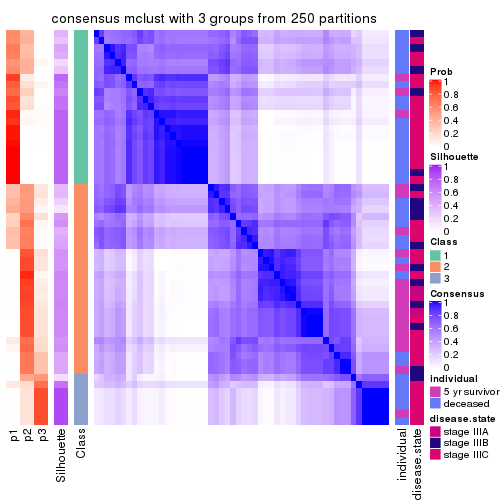
consensus_heatmap(res, k = 4)
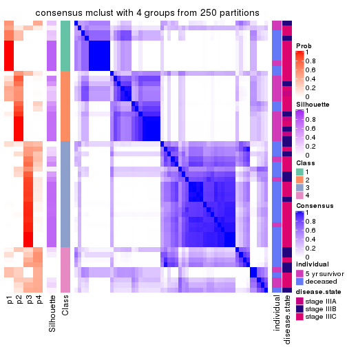
consensus_heatmap(res, k = 5)
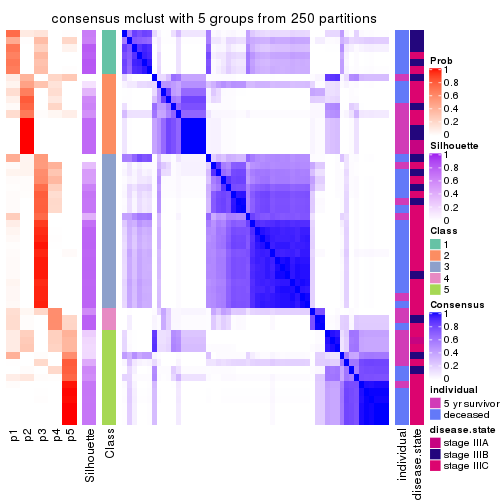
consensus_heatmap(res, k = 6)
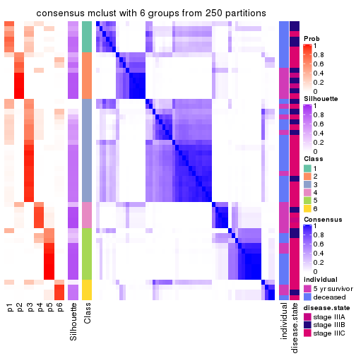
Heatmaps for the membership of samples in all partitions to see how consistent they are:
membership_heatmap(res, k = 2)
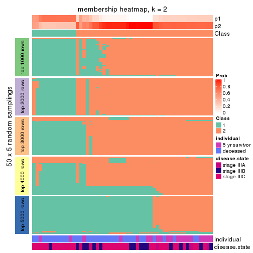
membership_heatmap(res, k = 3)
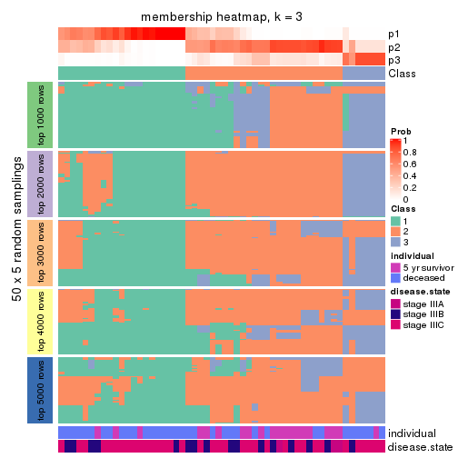
membership_heatmap(res, k = 4)
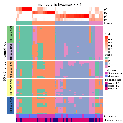
membership_heatmap(res, k = 5)
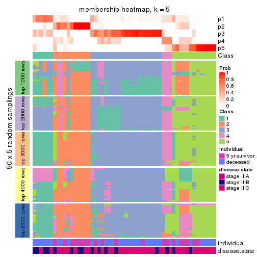
membership_heatmap(res, k = 6)
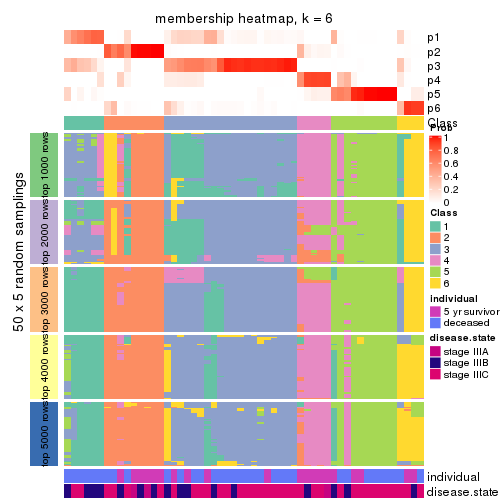
As soon as we have had the classes for columns, we can look for signatures which are significantly different between classes which can be candidate marks for certain classes. Following are the heatmaps for signatures.
Signature heatmaps where rows are scaled:
get_signatures(res, k = 2)
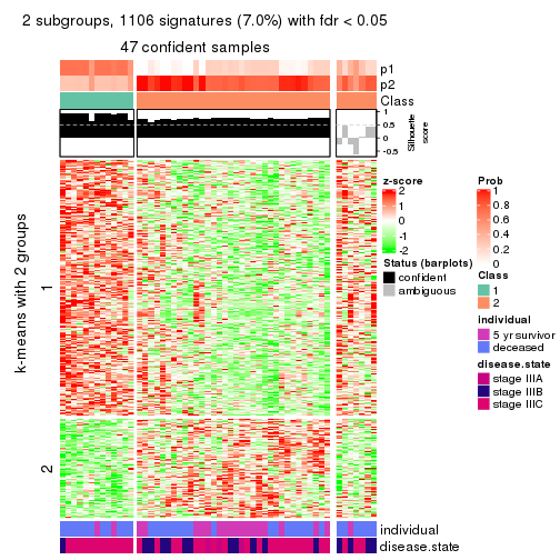
get_signatures(res, k = 3)
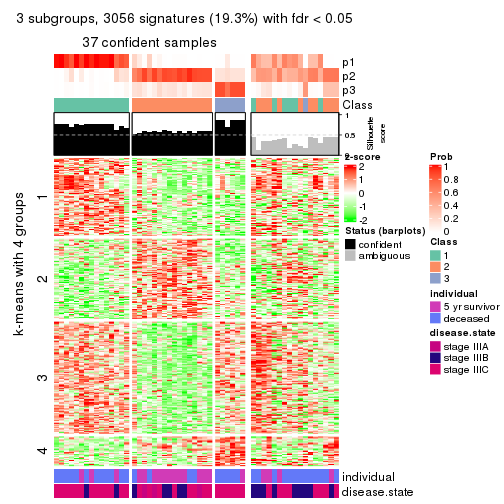
get_signatures(res, k = 4)
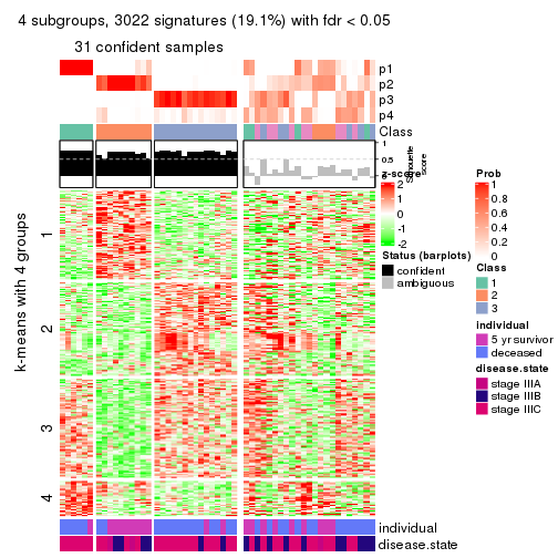
get_signatures(res, k = 5)
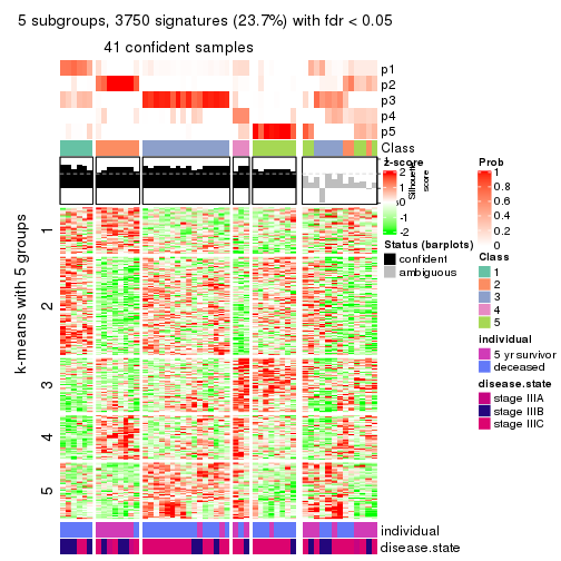
get_signatures(res, k = 6)
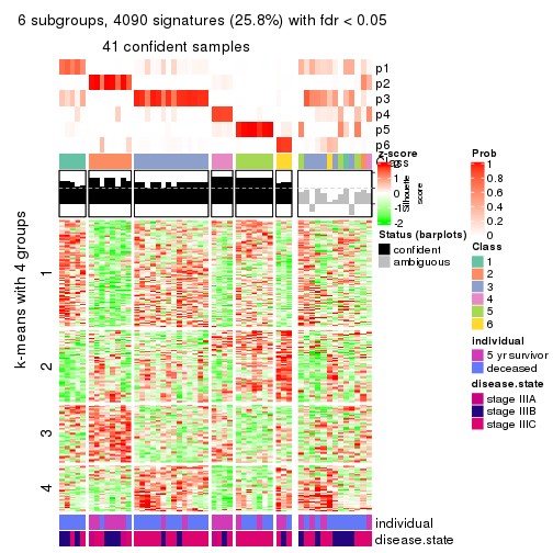
Signature heatmaps where rows are not scaled:
get_signatures(res, k = 2, scale_rows = FALSE)
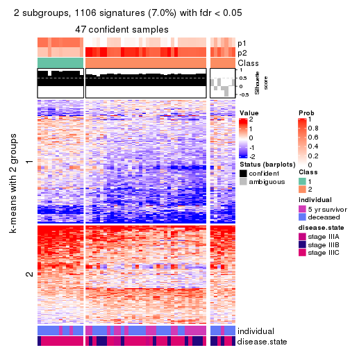
get_signatures(res, k = 3, scale_rows = FALSE)
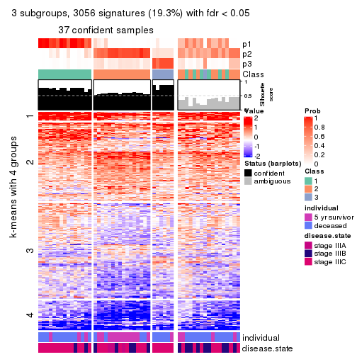
get_signatures(res, k = 4, scale_rows = FALSE)
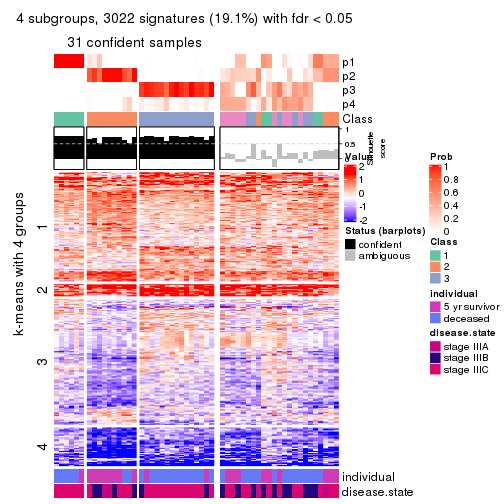
get_signatures(res, k = 5, scale_rows = FALSE)
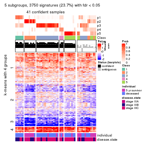
get_signatures(res, k = 6, scale_rows = FALSE)
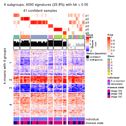
Compare the overlap of signatures from different k:
compare_signatures(res)
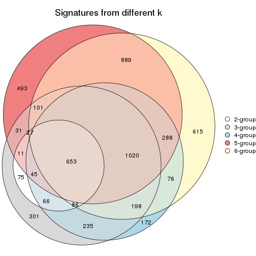
get_signature() returns a data frame invisibly. TO get the list of signatures, the function
call should be assigned to a variable explicitly. In following code, if plot argument is set
to FALSE, no heatmap is plotted while only the differential analysis is performed.
# code only for demonstration
tb = get_signature(res, k = ..., plot = FALSE)
An example of the output of tb is:
#>   which_row         fdr    mean_1    mean_2 scaled_mean_1 scaled_mean_2 km
#> 1        38 0.042760348  8.373488  9.131774    -0.5533452     0.5164555  1
#> 2        40 0.018707592  7.106213  8.469186    -0.6173731     0.5762149  1
#> 3        55 0.019134737 10.221463 11.207825    -0.6159697     0.5749050  1
#> 4        59 0.006059896  5.921854  7.869574    -0.6899429     0.6439467  1
#> 5        60 0.018055526  8.928898 10.211722    -0.6204761     0.5791110  1
#> 6        98 0.009384629 15.714769 14.887706     0.6635654    -0.6193277  2
...
The columns in tb are:
which_row: row indices corresponding to the input matrix.fdr: FDR for the differential test. mean_x: The mean value in group x.scaled_mean_x: The mean value in group x after rows are scaled.km: Row groups if k-means clustering is applied to rows.UMAP plot which shows how samples are separated.
dimension_reduction(res, k = 2, method = "UMAP")
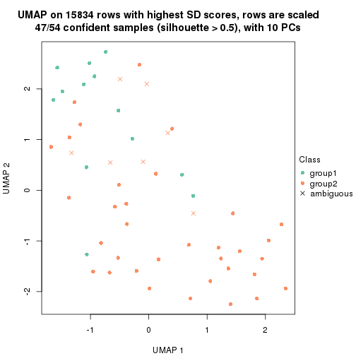
dimension_reduction(res, k = 3, method = "UMAP")
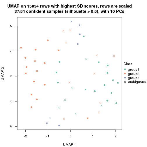
dimension_reduction(res, k = 4, method = "UMAP")
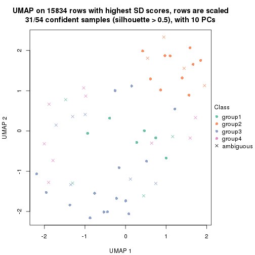
dimension_reduction(res, k = 5, method = "UMAP")
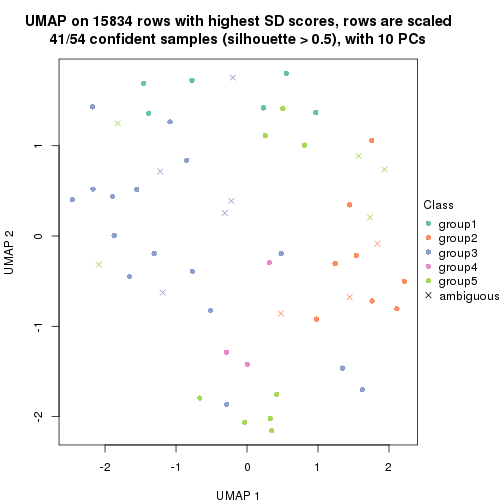
dimension_reduction(res, k = 6, method = "UMAP")
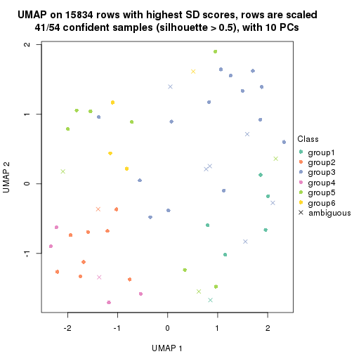
Following heatmap shows how subgroups are split when increasing k:
collect_classes(res)
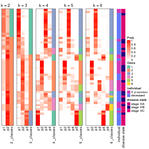
Test correlation between subgroups and known annotations. If the known annotation is numeric, one-way ANOVA test is applied, and if the known annotation is discrete, chi-squared contingency table test is applied.
test_to_known_factors(res)
#>            n individual(p) disease.state(p) k
#> SD:mclust 47      0.067124           0.0848 2
#> SD:mclust 37      0.003023           0.0677 3
#> SD:mclust 31      0.001662           0.0361 4
#> SD:mclust 41      0.000336           0.0457 5
#> SD:mclust 41      0.002198           0.0900 6
If matrix rows can be associated to genes, consider to use functional_enrichment(res,
...) to perform function enrichment for the signature genes. See this vignette for more detailed explanations.
The object with results only for a single top-value method and a single partition method can be extracted as:
res = res_list["SD", "NMF"]
# you can also extract it by
# res = res_list["SD:NMF"]
A summary of res and all the functions that can be applied to it:
res
#> A 'ConsensusPartition' object with k = 2, 3, 4, 5, 6.
#>   On a matrix with 15834 rows and 54 columns.
#>   Top rows (1000, 2000, 3000, 4000, 5000) are extracted by 'SD' method.
#>   Subgroups are detected by 'NMF' method.
#>   Performed in total 1250 partitions by row resampling.
#>   Best k for subgroups seems to be 2.
#>
#> Following methods can be applied to this 'ConsensusPartition' object:
#>  [1] "cola_report"             "collect_classes"         "collect_plots"
#>  [4] "collect_stats"           "colnames"                "compare_signatures"
#>  [7] "consensus_heatmap"       "dimension_reduction"     "functional_enrichment"
#> [10] "get_anno_col"            "get_anno"                "get_classes"
#> [13] "get_consensus"           "get_matrix"              "get_membership"
#> [16] "get_param"               "get_signatures"          "get_stats"
#> [19] "is_best_k"               "is_stable_k"             "membership_heatmap"
#> [22] "ncol"                    "nrow"                    "plot_ecdf"
#> [25] "rownames"                "select_partition_number" "show"
#> [28] "suggest_best_k"          "test_to_known_factors"
collect_plots() function collects all the plots made from res for all k (number of partitions)
into one single page to provide an easy and fast comparison between different k.
collect_plots(res)
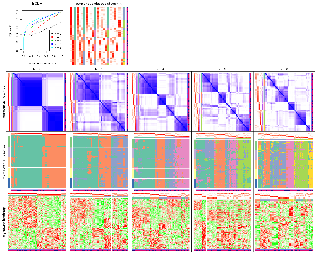
The plots are:
k and the heatmap of
predicted classes for each k.k.k.k.All the plots in panels can be made by individual functions and they are plotted later in this section.
select_partition_number() produces several plots showing different
statistics for choosing “optimized” k. There are following statistics:
k;k, the area increased is defined as \(A_k - A_{k-1}\).The detailed explanations of these statistics can be found in the cola vignette.
Generally speaking, lower PAC score, higher mean silhouette score or higher
concordance corresponds to better partition. Rand index and Jaccard index
measure how similar the current partition is compared to partition with k-1.
If they are too similar, we won't accept k is better than k-1.
select_partition_number(res)
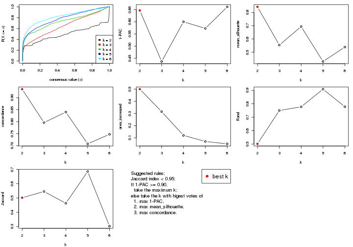
The numeric values for all these statistics can be obtained by get_stats().
get_stats(res)
#>   k 1-PAC mean_silhouette concordance area_increased  Rand Jaccard
#> 2 2 0.646           0.842       0.935         0.4995 0.502   0.502
#> 3 3 0.437           0.554       0.796         0.3150 0.750   0.545
#> 4 4 0.600           0.694       0.840         0.1199 0.777   0.463
#> 5 5 0.573           0.430       0.708         0.0701 0.908   0.685
#> 6 6 0.661           0.539       0.747         0.0506 0.778   0.303
suggest_best_k() suggests the best \(k\) based on these statistics. The rules are as follows:
suggest_best_k(res)
#> [1] 2
Following shows the table of the partitions (You need to click the show/hide
code output link to see it). The membership matrix (columns with name p*)
is inferred by
clue::cl_consensus()
function with the SE method. Basically the value in the membership matrix
represents the probability to belong to a certain group. The finall class
label for an item is determined with the group with highest probability it
belongs to.
In get_classes() function, the entropy is calculated from the membership
matrix and the silhouette score is calculated from the consensus matrix.
cbind(get_classes(res, k = 2), get_membership(res, k = 2))
#>           class entropy silhouette    p1    p2
#> GSM311939     2  0.0376     0.9389 0.004 0.996
#> GSM311963     2  0.0376     0.9389 0.004 0.996
#> GSM311973     2  0.6048     0.8149 0.148 0.852
#> GSM311940     2  0.0000     0.9375 0.000 1.000
#> GSM311953     2  0.0376     0.9389 0.004 0.996
#> GSM311974     2  0.0376     0.9389 0.004 0.996
#> GSM311975     1  0.0672     0.9130 0.992 0.008
#> GSM311977     2  0.0376     0.9389 0.004 0.996
#> GSM311982     1  0.0000     0.9161 1.000 0.000
#> GSM311990     2  0.0000     0.9375 0.000 1.000
#> GSM311943     1  0.0000     0.9161 1.000 0.000
#> GSM311944     1  0.0000     0.9161 1.000 0.000
#> GSM311946     2  0.0376     0.9389 0.004 0.996
#> GSM311956     2  0.0376     0.9389 0.004 0.996
#> GSM311967     2  0.0000     0.9375 0.000 1.000
#> GSM311968     2  0.0672     0.9373 0.008 0.992
#> GSM311972     1  0.0000     0.9161 1.000 0.000
#> GSM311980     2  0.5059     0.8550 0.112 0.888
#> GSM311981     1  0.9732     0.3137 0.596 0.404
#> GSM311988     2  0.0376     0.9389 0.004 0.996
#> GSM311957     1  0.0000     0.9161 1.000 0.000
#> GSM311960     1  0.0938     0.9088 0.988 0.012
#> GSM311971     1  0.5059     0.8171 0.888 0.112
#> GSM311976     1  0.0000     0.9161 1.000 0.000
#> GSM311978     1  0.0000     0.9161 1.000 0.000
#> GSM311979     1  0.0000     0.9161 1.000 0.000
#> GSM311983     1  0.0000     0.9161 1.000 0.000
#> GSM311986     2  0.7815     0.6976 0.232 0.768
#> GSM311991     1  0.1414     0.9052 0.980 0.020
#> GSM311938     2  0.0376     0.9389 0.004 0.996
#> GSM311941     1  0.4939     0.8252 0.892 0.108
#> GSM311942     1  0.9944     0.1616 0.544 0.456
#> GSM311945     1  0.0000     0.9161 1.000 0.000
#> GSM311947     2  0.0000     0.9375 0.000 1.000
#> GSM311948     2  0.0672     0.9373 0.008 0.992
#> GSM311949     1  0.0000     0.9161 1.000 0.000
#> GSM311950     2  0.0000     0.9375 0.000 1.000
#> GSM311951     1  0.7745     0.6747 0.772 0.228
#> GSM311952     1  0.0000     0.9161 1.000 0.000
#> GSM311954     2  0.8713     0.5899 0.292 0.708
#> GSM311955     1  0.0000     0.9161 1.000 0.000
#> GSM311958     1  0.0376     0.9138 0.996 0.004
#> GSM311959     1  0.9909     0.2050 0.556 0.444
#> GSM311961     1  0.0000     0.9161 1.000 0.000
#> GSM311962     1  0.0000     0.9161 1.000 0.000
#> GSM311964     1  0.0000     0.9161 1.000 0.000
#> GSM311965     2  0.7376     0.7342 0.208 0.792
#> GSM311966     1  0.0000     0.9161 1.000 0.000
#> GSM311969     1  0.0376     0.9142 0.996 0.004
#> GSM311970     2  0.0376     0.9370 0.004 0.996
#> GSM311984     1  0.9983     0.0887 0.524 0.476
#> GSM311985     1  0.0000     0.9161 1.000 0.000
#> GSM311987     2  0.6623     0.7822 0.172 0.828
#> GSM311989     1  0.0376     0.9138 0.996 0.004
cbind(get_classes(res, k = 3), get_membership(res, k = 3))
#>           class entropy silhouette    p1    p2    p3
#> GSM311939     3  0.6308     0.1862 0.000 0.492 0.508
#> GSM311963     3  0.6244     0.3020 0.000 0.440 0.560
#> GSM311973     2  0.0848     0.7089 0.008 0.984 0.008
#> GSM311940     3  0.6026     0.3954 0.000 0.376 0.624
#> GSM311953     2  0.3816     0.6093 0.000 0.852 0.148
#> GSM311974     2  0.2796     0.6772 0.000 0.908 0.092
#> GSM311975     1  0.6215     0.2426 0.572 0.000 0.428
#> GSM311977     2  0.6308    -0.2652 0.000 0.508 0.492
#> GSM311982     1  0.4750     0.6904 0.784 0.216 0.000
#> GSM311990     3  0.6180     0.0273 0.000 0.416 0.584
#> GSM311943     1  0.1163     0.8087 0.972 0.000 0.028
#> GSM311944     1  0.5529     0.5857 0.704 0.296 0.000
#> GSM311946     2  0.4504     0.5425 0.000 0.804 0.196
#> GSM311956     2  0.2261     0.6885 0.000 0.932 0.068
#> GSM311967     3  0.0829     0.5967 0.012 0.004 0.984
#> GSM311968     2  0.3532     0.6877 0.008 0.884 0.108
#> GSM311972     1  0.1860     0.8052 0.948 0.052 0.000
#> GSM311980     2  0.0661     0.7090 0.008 0.988 0.004
#> GSM311981     3  0.6189     0.3130 0.364 0.004 0.632
#> GSM311988     3  0.6026     0.3749 0.000 0.376 0.624
#> GSM311957     1  0.2261     0.8008 0.932 0.068 0.000
#> GSM311960     2  0.5216     0.5225 0.260 0.740 0.000
#> GSM311971     1  0.5835     0.5023 0.660 0.340 0.000
#> GSM311976     1  0.2031     0.8087 0.952 0.016 0.032
#> GSM311978     1  0.2537     0.7985 0.920 0.080 0.000
#> GSM311979     1  0.3192     0.7781 0.888 0.112 0.000
#> GSM311983     1  0.1643     0.8027 0.956 0.000 0.044
#> GSM311986     3  0.5138     0.5165 0.252 0.000 0.748
#> GSM311991     1  0.6809     0.0800 0.524 0.012 0.464
#> GSM311938     3  0.2680     0.5943 0.008 0.068 0.924
#> GSM311941     1  0.4555     0.6741 0.800 0.000 0.200
#> GSM311942     2  0.6910     0.5730 0.120 0.736 0.144
#> GSM311945     1  0.6168     0.3650 0.588 0.412 0.000
#> GSM311947     3  0.6148     0.1556 0.004 0.356 0.640
#> GSM311948     2  0.3120     0.7054 0.012 0.908 0.080
#> GSM311949     1  0.1765     0.8100 0.956 0.040 0.004
#> GSM311950     3  0.2959     0.5794 0.000 0.100 0.900
#> GSM311951     2  0.6924     0.1341 0.400 0.580 0.020
#> GSM311952     1  0.0747     0.8101 0.984 0.000 0.016
#> GSM311954     3  0.3482     0.5911 0.128 0.000 0.872
#> GSM311955     1  0.5363     0.5560 0.724 0.000 0.276
#> GSM311958     1  0.2066     0.7959 0.940 0.000 0.060
#> GSM311959     3  0.4702     0.5595 0.212 0.000 0.788
#> GSM311961     1  0.2261     0.7924 0.932 0.000 0.068
#> GSM311962     1  0.1163     0.8074 0.972 0.000 0.028
#> GSM311964     1  0.2625     0.7945 0.916 0.084 0.000
#> GSM311965     2  0.5307     0.6484 0.056 0.820 0.124
#> GSM311966     1  0.0747     0.8100 0.984 0.000 0.016
#> GSM311969     1  0.3192     0.7656 0.888 0.000 0.112
#> GSM311970     3  0.6421     0.3073 0.004 0.424 0.572
#> GSM311984     3  0.6295     0.0226 0.472 0.000 0.528
#> GSM311985     1  0.0829     0.8106 0.984 0.004 0.012
#> GSM311987     3  0.2878     0.5966 0.096 0.000 0.904
#> GSM311989     1  0.6154     0.3713 0.592 0.408 0.000
cbind(get_classes(res, k = 4), get_membership(res, k = 4))
#>           class entropy silhouette    p1    p2    p3    p4
#> GSM311939     2  0.0779      0.860 0.000 0.980 0.016 0.004
#> GSM311963     2  0.0188      0.860 0.000 0.996 0.000 0.004
#> GSM311973     4  0.5097      0.373 0.004 0.428 0.000 0.568
#> GSM311940     2  0.1576      0.844 0.000 0.948 0.048 0.004
#> GSM311953     2  0.1807      0.841 0.000 0.940 0.008 0.052
#> GSM311974     4  0.5658      0.507 0.000 0.328 0.040 0.632
#> GSM311975     3  0.5070      0.508 0.372 0.008 0.620 0.000
#> GSM311977     2  0.0336      0.860 0.000 0.992 0.000 0.008
#> GSM311982     4  0.4477      0.530 0.312 0.000 0.000 0.688
#> GSM311990     3  0.5364      0.334 0.000 0.028 0.652 0.320
#> GSM311943     1  0.1362      0.827 0.964 0.004 0.020 0.012
#> GSM311944     4  0.3942      0.636 0.236 0.000 0.000 0.764
#> GSM311946     2  0.1452      0.852 0.000 0.956 0.008 0.036
#> GSM311956     4  0.3300      0.769 0.000 0.144 0.008 0.848
#> GSM311967     3  0.0524      0.610 0.004 0.008 0.988 0.000
#> GSM311968     4  0.0937      0.813 0.000 0.012 0.012 0.976
#> GSM311972     1  0.1297      0.825 0.964 0.000 0.016 0.020
#> GSM311980     4  0.3300      0.770 0.008 0.144 0.000 0.848
#> GSM311981     3  0.5322      0.586 0.312 0.028 0.660 0.000
#> GSM311988     2  0.0707      0.859 0.000 0.980 0.020 0.000
#> GSM311957     1  0.2654      0.772 0.888 0.004 0.000 0.108
#> GSM311960     4  0.1576      0.816 0.048 0.004 0.000 0.948
#> GSM311971     1  0.7269      0.319 0.524 0.296 0.000 0.180
#> GSM311976     1  0.1975      0.813 0.936 0.048 0.016 0.000
#> GSM311978     1  0.2021      0.808 0.932 0.012 0.000 0.056
#> GSM311979     1  0.3942      0.642 0.764 0.000 0.000 0.236
#> GSM311983     1  0.1492      0.819 0.956 0.004 0.036 0.004
#> GSM311986     3  0.5856      0.572 0.240 0.056 0.692 0.012
#> GSM311991     3  0.6374      0.478 0.372 0.072 0.556 0.000
#> GSM311938     2  0.4455      0.709 0.024 0.800 0.164 0.012
#> GSM311941     1  0.5713      0.385 0.620 0.000 0.340 0.040
#> GSM311942     4  0.0376      0.815 0.004 0.004 0.000 0.992
#> GSM311945     4  0.2216      0.794 0.092 0.000 0.000 0.908
#> GSM311947     3  0.4122      0.481 0.000 0.004 0.760 0.236
#> GSM311948     4  0.3958      0.747 0.000 0.160 0.024 0.816
#> GSM311949     1  0.2730      0.784 0.896 0.088 0.000 0.016
#> GSM311950     2  0.5155      0.216 0.000 0.528 0.468 0.004
#> GSM311951     4  0.0817      0.818 0.024 0.000 0.000 0.976
#> GSM311952     1  0.0712      0.827 0.984 0.004 0.008 0.004
#> GSM311954     3  0.5297      0.590 0.292 0.032 0.676 0.000
#> GSM311955     1  0.4077      0.662 0.800 0.012 0.184 0.004
#> GSM311958     1  0.1792      0.807 0.932 0.000 0.068 0.000
#> GSM311959     3  0.4360      0.655 0.248 0.008 0.744 0.000
#> GSM311961     1  0.1888      0.814 0.940 0.016 0.044 0.000
#> GSM311962     1  0.1082      0.825 0.972 0.004 0.020 0.004
#> GSM311964     1  0.3852      0.693 0.800 0.000 0.008 0.192
#> GSM311965     4  0.0844      0.814 0.004 0.004 0.012 0.980
#> GSM311966     1  0.0188      0.826 0.996 0.000 0.000 0.004
#> GSM311969     1  0.3272      0.747 0.860 0.004 0.128 0.008
#> GSM311970     2  0.4343      0.622 0.000 0.732 0.264 0.004
#> GSM311984     1  0.6515      0.465 0.672 0.156 0.160 0.012
#> GSM311985     1  0.0927      0.827 0.976 0.000 0.016 0.008
#> GSM311987     3  0.2495      0.616 0.028 0.036 0.924 0.012
#> GSM311989     4  0.1389      0.814 0.048 0.000 0.000 0.952
cbind(get_classes(res, k = 5), get_membership(res, k = 5))
#>           class entropy silhouette    p1    p2    p3    p4    p5
#> GSM311939     2  0.1386     0.7998 0.032 0.952 0.016 0.000 0.000
#> GSM311963     2  0.0613     0.8049 0.008 0.984 0.004 0.004 0.000
#> GSM311973     2  0.5422     0.4491 0.000 0.616 0.072 0.004 0.308
#> GSM311940     2  0.3682     0.7277 0.000 0.820 0.072 0.108 0.000
#> GSM311953     2  0.1732     0.7891 0.000 0.920 0.000 0.000 0.080
#> GSM311974     5  0.3579     0.4986 0.000 0.240 0.004 0.000 0.756
#> GSM311975     4  0.4575     0.4158 0.328 0.000 0.024 0.648 0.000
#> GSM311977     2  0.1907     0.7889 0.000 0.928 0.044 0.028 0.000
#> GSM311982     5  0.6632     0.0945 0.344 0.000 0.228 0.000 0.428
#> GSM311990     5  0.5896     0.2300 0.000 0.000 0.448 0.100 0.452
#> GSM311943     1  0.0932     0.4735 0.972 0.004 0.004 0.020 0.000
#> GSM311944     5  0.6149     0.3310 0.372 0.000 0.064 0.032 0.532
#> GSM311946     2  0.1830     0.8015 0.028 0.932 0.000 0.000 0.040
#> GSM311956     5  0.0771     0.6875 0.000 0.020 0.000 0.004 0.976
#> GSM311967     4  0.2728     0.6500 0.000 0.004 0.068 0.888 0.040
#> GSM311968     5  0.0451     0.6879 0.000 0.008 0.004 0.000 0.988
#> GSM311972     1  0.6894     0.2874 0.420 0.000 0.364 0.204 0.012
#> GSM311980     5  0.3010     0.6530 0.000 0.116 0.016 0.008 0.860
#> GSM311981     4  0.1554     0.6741 0.024 0.008 0.012 0.952 0.004
#> GSM311988     2  0.2074     0.7829 0.036 0.920 0.044 0.000 0.000
#> GSM311957     1  0.5512     0.3586 0.560 0.040 0.384 0.000 0.016
#> GSM311960     5  0.4526     0.5569 0.028 0.000 0.300 0.000 0.672
#> GSM311971     3  0.7056    -0.3396 0.404 0.160 0.404 0.000 0.032
#> GSM311976     1  0.7814     0.2277 0.436 0.136 0.300 0.128 0.000
#> GSM311978     1  0.4696     0.3751 0.584 0.004 0.400 0.000 0.012
#> GSM311979     1  0.5408     0.3243 0.532 0.000 0.408 0.000 0.060
#> GSM311983     1  0.1967     0.4635 0.932 0.012 0.020 0.036 0.000
#> GSM311986     3  0.6560    -0.0558 0.380 0.092 0.492 0.036 0.000
#> GSM311991     4  0.2519     0.6678 0.100 0.000 0.016 0.884 0.000
#> GSM311938     2  0.4135     0.7129 0.064 0.820 0.072 0.044 0.000
#> GSM311941     3  0.5739    -0.3638 0.432 0.000 0.504 0.020 0.044
#> GSM311942     5  0.3075     0.6817 0.092 0.000 0.048 0.000 0.860
#> GSM311945     5  0.5450     0.5458 0.124 0.000 0.228 0.000 0.648
#> GSM311947     5  0.6612     0.0938 0.000 0.000 0.248 0.296 0.456
#> GSM311948     5  0.2411     0.6475 0.000 0.108 0.008 0.000 0.884
#> GSM311949     1  0.5076     0.3831 0.592 0.028 0.372 0.000 0.008
#> GSM311950     4  0.5605    -0.0832 0.000 0.404 0.076 0.520 0.000
#> GSM311951     5  0.3966     0.6594 0.132 0.000 0.072 0.000 0.796
#> GSM311952     1  0.0865     0.4733 0.972 0.024 0.004 0.000 0.000
#> GSM311954     4  0.6551     0.4611 0.132 0.040 0.244 0.584 0.000
#> GSM311955     1  0.3882     0.3730 0.824 0.016 0.060 0.100 0.000
#> GSM311958     1  0.4793     0.3596 0.684 0.000 0.056 0.260 0.000
#> GSM311959     4  0.3779     0.6557 0.116 0.012 0.048 0.824 0.000
#> GSM311961     1  0.4256     0.3793 0.796 0.068 0.016 0.120 0.000
#> GSM311962     1  0.1216     0.4862 0.960 0.000 0.020 0.020 0.000
#> GSM311964     1  0.5854     0.3109 0.516 0.000 0.408 0.016 0.060
#> GSM311965     5  0.0609     0.6876 0.000 0.000 0.020 0.000 0.980
#> GSM311966     1  0.4360     0.4376 0.680 0.000 0.300 0.020 0.000
#> GSM311969     1  0.3690     0.3630 0.828 0.008 0.112 0.052 0.000
#> GSM311970     2  0.5626     0.1800 0.000 0.504 0.076 0.420 0.000
#> GSM311984     1  0.6258    -0.0377 0.564 0.216 0.216 0.004 0.000
#> GSM311985     1  0.5901     0.4004 0.568 0.000 0.300 0.132 0.000
#> GSM311987     3  0.6512    -0.4120 0.108 0.016 0.480 0.392 0.004
#> GSM311989     5  0.4774     0.6429 0.112 0.000 0.132 0.008 0.748
cbind(get_classes(res, k = 6), get_membership(res, k = 6))
#>           class entropy silhouette    p1    p2    p3    p4    p5    p6
#> GSM311939     2  0.0748     0.7479 0.016 0.976 0.004 0.000 0.000 0.004
#> GSM311963     2  0.1806     0.7217 0.088 0.908 0.000 0.000 0.000 0.004
#> GSM311973     4  0.4651     0.5960 0.084 0.212 0.000 0.696 0.004 0.004
#> GSM311940     1  0.4627    -0.1885 0.512 0.456 0.000 0.008 0.000 0.024
#> GSM311953     4  0.4127     0.2907 0.004 0.400 0.000 0.588 0.000 0.008
#> GSM311974     4  0.1082     0.8539 0.004 0.040 0.000 0.956 0.000 0.000
#> GSM311975     3  0.3775     0.5783 0.092 0.000 0.780 0.000 0.000 0.128
#> GSM311977     2  0.3733     0.4929 0.288 0.700 0.000 0.008 0.000 0.004
#> GSM311982     5  0.4368     0.4464 0.000 0.000 0.016 0.384 0.592 0.008
#> GSM311990     6  0.2431     0.6565 0.008 0.000 0.000 0.132 0.000 0.860
#> GSM311943     3  0.4501     0.4097 0.000 0.012 0.660 0.000 0.292 0.036
#> GSM311944     5  0.7553     0.1100 0.000 0.000 0.192 0.288 0.336 0.184
#> GSM311946     2  0.4560     0.4934 0.012 0.680 0.032 0.268 0.000 0.008
#> GSM311956     4  0.0260     0.8591 0.000 0.008 0.000 0.992 0.000 0.000
#> GSM311967     6  0.4047     0.4108 0.384 0.000 0.012 0.000 0.000 0.604
#> GSM311968     4  0.0520     0.8499 0.000 0.000 0.000 0.984 0.008 0.008
#> GSM311972     3  0.5407     0.4811 0.216 0.008 0.624 0.000 0.148 0.004
#> GSM311980     4  0.0982     0.8596 0.004 0.020 0.000 0.968 0.004 0.004
#> GSM311981     1  0.5029    -0.2003 0.524 0.000 0.400 0.000 0.000 0.076
#> GSM311988     2  0.0725     0.7471 0.012 0.976 0.000 0.000 0.000 0.012
#> GSM311957     5  0.0260     0.7909 0.000 0.000 0.008 0.000 0.992 0.000
#> GSM311960     5  0.1265     0.7940 0.000 0.000 0.000 0.044 0.948 0.008
#> GSM311971     5  0.1327     0.7780 0.000 0.064 0.000 0.000 0.936 0.000
#> GSM311976     1  0.6605     0.1978 0.484 0.084 0.092 0.000 0.332 0.008
#> GSM311978     5  0.1364     0.7906 0.016 0.020 0.012 0.000 0.952 0.000
#> GSM311979     5  0.0000     0.7923 0.000 0.000 0.000 0.000 1.000 0.000
#> GSM311983     3  0.2665     0.6343 0.000 0.060 0.884 0.000 0.032 0.024
#> GSM311986     6  0.3867     0.5511 0.004 0.036 0.216 0.000 0.000 0.744
#> GSM311991     3  0.5418     0.1881 0.388 0.000 0.492 0.000 0.000 0.120
#> GSM311938     2  0.4272     0.5815 0.148 0.772 0.032 0.012 0.000 0.036
#> GSM311941     5  0.5234     0.0382 0.052 0.000 0.020 0.000 0.520 0.408
#> GSM311942     5  0.2988     0.7577 0.000 0.000 0.000 0.144 0.828 0.028
#> GSM311945     5  0.2039     0.7866 0.000 0.000 0.000 0.076 0.904 0.020
#> GSM311947     6  0.2888     0.6730 0.056 0.000 0.000 0.092 0.000 0.852
#> GSM311948     4  0.1149     0.8567 0.008 0.024 0.008 0.960 0.000 0.000
#> GSM311949     5  0.1760     0.7744 0.004 0.048 0.020 0.000 0.928 0.000
#> GSM311950     1  0.4482     0.2964 0.708 0.168 0.000 0.000 0.000 0.124
#> GSM311951     5  0.3942     0.7375 0.000 0.000 0.008 0.120 0.780 0.092
#> GSM311952     3  0.4641     0.5054 0.000 0.192 0.696 0.000 0.108 0.004
#> GSM311954     1  0.7263    -0.1127 0.392 0.088 0.244 0.000 0.004 0.272
#> GSM311955     3  0.3588     0.6235 0.084 0.052 0.832 0.000 0.008 0.024
#> GSM311958     3  0.5046     0.5483 0.172 0.000 0.700 0.000 0.068 0.060
#> GSM311959     3  0.5821     0.1268 0.392 0.000 0.444 0.000 0.004 0.160
#> GSM311961     3  0.2588     0.6132 0.004 0.124 0.860 0.000 0.000 0.012
#> GSM311962     3  0.2676     0.6373 0.004 0.056 0.880 0.000 0.056 0.004
#> GSM311964     5  0.0000     0.7923 0.000 0.000 0.000 0.000 1.000 0.000
#> GSM311965     4  0.1088     0.8409 0.000 0.000 0.000 0.960 0.024 0.016
#> GSM311966     3  0.4622     0.5739 0.092 0.008 0.716 0.000 0.180 0.004
#> GSM311969     3  0.2847     0.6311 0.000 0.036 0.876 0.000 0.040 0.048
#> GSM311970     1  0.4594     0.2413 0.676 0.232 0.000 0.000 0.000 0.092
#> GSM311984     3  0.4263     0.0600 0.000 0.480 0.504 0.000 0.000 0.016
#> GSM311985     3  0.4890     0.5542 0.164 0.000 0.708 0.000 0.096 0.032
#> GSM311987     6  0.3618     0.6006 0.176 0.000 0.048 0.000 0.000 0.776
#> GSM311989     5  0.4719     0.6507 0.000 0.000 0.012 0.080 0.688 0.220
Heatmaps for the consensus matrix. It visualizes the probability of two samples to be in a same group.
consensus_heatmap(res, k = 2)
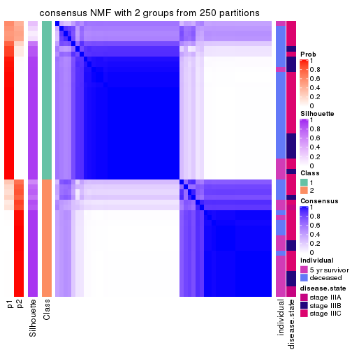
consensus_heatmap(res, k = 3)
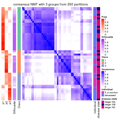
consensus_heatmap(res, k = 4)
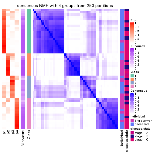
consensus_heatmap(res, k = 5)
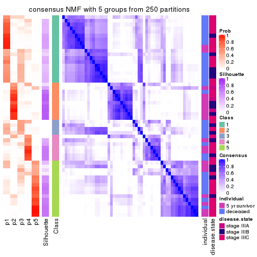
consensus_heatmap(res, k = 6)
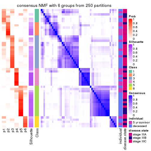
Heatmaps for the membership of samples in all partitions to see how consistent they are:
membership_heatmap(res, k = 2)
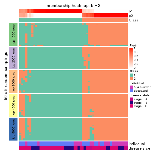
membership_heatmap(res, k = 3)
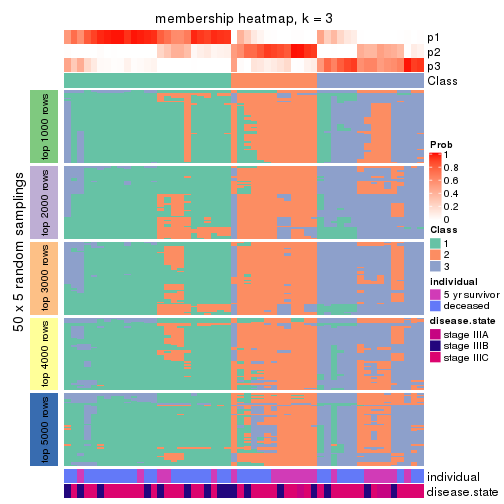
membership_heatmap(res, k = 4)
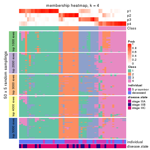
membership_heatmap(res, k = 5)
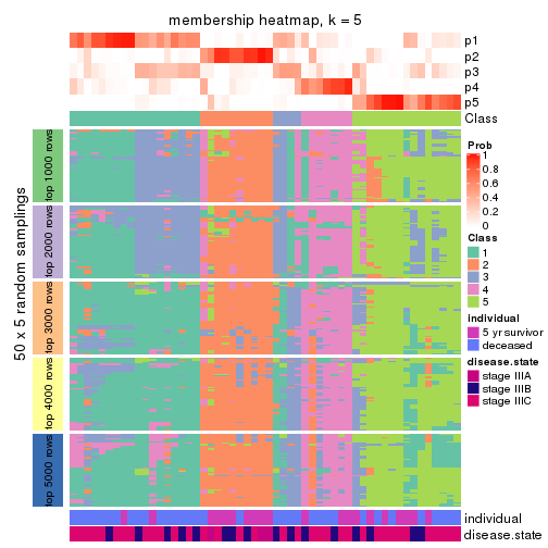
membership_heatmap(res, k = 6)
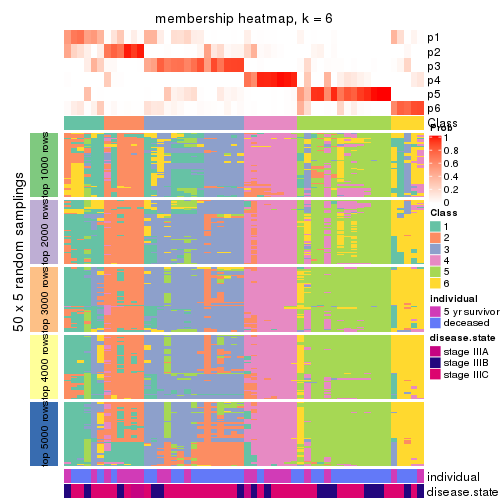
As soon as we have had the classes for columns, we can look for signatures which are significantly different between classes which can be candidate marks for certain classes. Following are the heatmaps for signatures.
Signature heatmaps where rows are scaled:
get_signatures(res, k = 2)
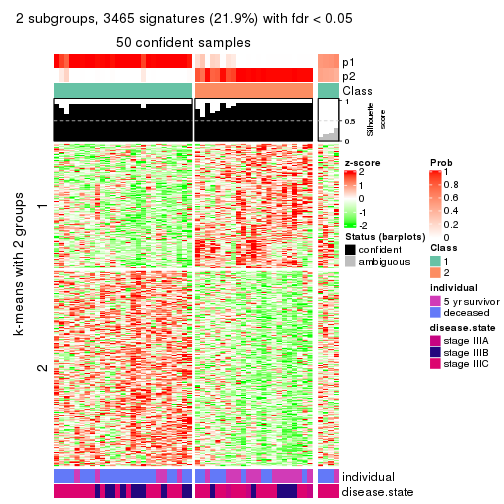
get_signatures(res, k = 3)
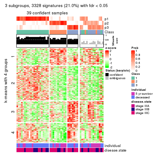
get_signatures(res, k = 4)
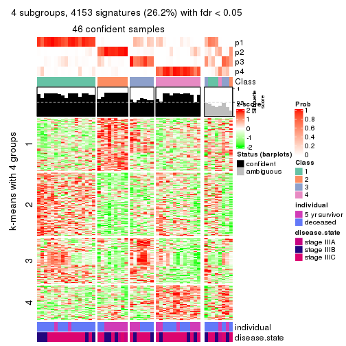
get_signatures(res, k = 5)
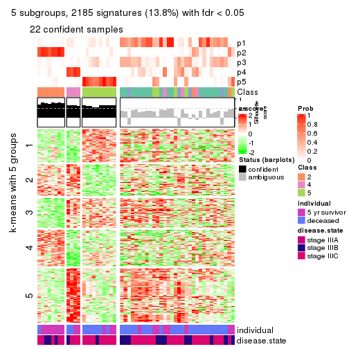
get_signatures(res, k = 6)
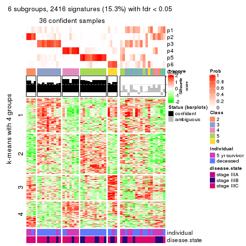
Signature heatmaps where rows are not scaled:
get_signatures(res, k = 2, scale_rows = FALSE)
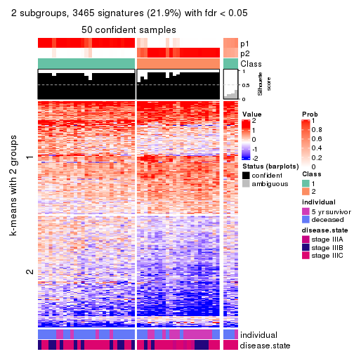
get_signatures(res, k = 3, scale_rows = FALSE)
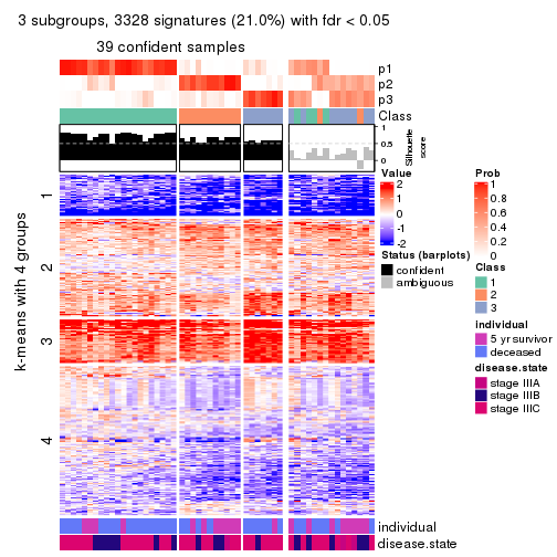
get_signatures(res, k = 4, scale_rows = FALSE)
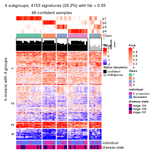
get_signatures(res, k = 5, scale_rows = FALSE)
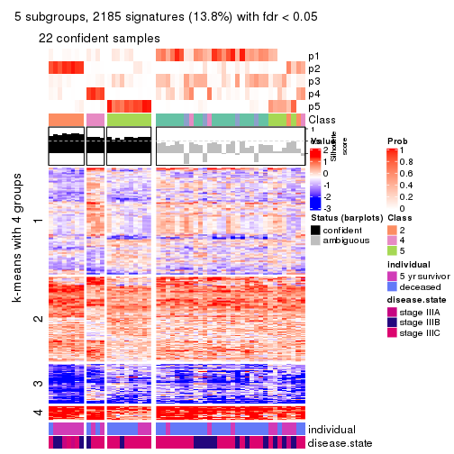
get_signatures(res, k = 6, scale_rows = FALSE)
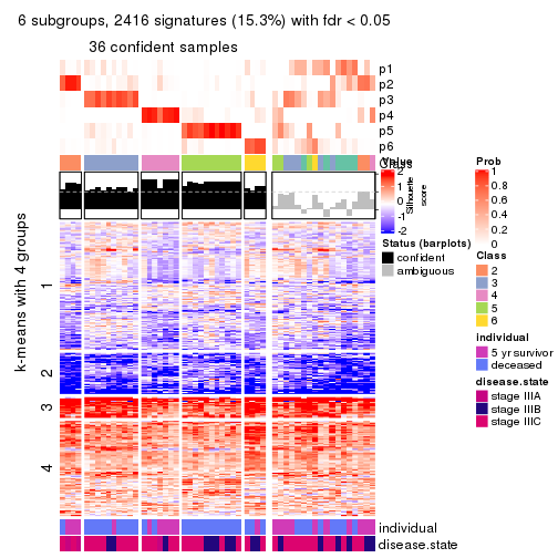
Compare the overlap of signatures from different k:
compare_signatures(res)
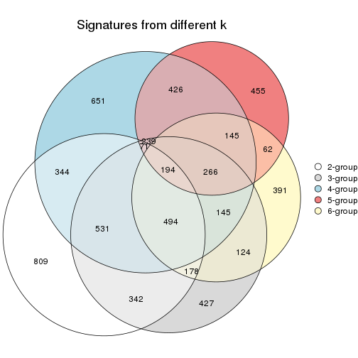
get_signature() returns a data frame invisibly. TO get the list of signatures, the function
call should be assigned to a variable explicitly. In following code, if plot argument is set
to FALSE, no heatmap is plotted while only the differential analysis is performed.
# code only for demonstration
tb = get_signature(res, k = ..., plot = FALSE)
An example of the output of tb is:
#>   which_row         fdr    mean_1    mean_2 scaled_mean_1 scaled_mean_2 km
#> 1        38 0.042760348  8.373488  9.131774    -0.5533452     0.5164555  1
#> 2        40 0.018707592  7.106213  8.469186    -0.6173731     0.5762149  1
#> 3        55 0.019134737 10.221463 11.207825    -0.6159697     0.5749050  1
#> 4        59 0.006059896  5.921854  7.869574    -0.6899429     0.6439467  1
#> 5        60 0.018055526  8.928898 10.211722    -0.6204761     0.5791110  1
#> 6        98 0.009384629 15.714769 14.887706     0.6635654    -0.6193277  2
...
The columns in tb are:
which_row: row indices corresponding to the input matrix.fdr: FDR for the differential test. mean_x: The mean value in group x.scaled_mean_x: The mean value in group x after rows are scaled.km: Row groups if k-means clustering is applied to rows.UMAP plot which shows how samples are separated.
dimension_reduction(res, k = 2, method = "UMAP")
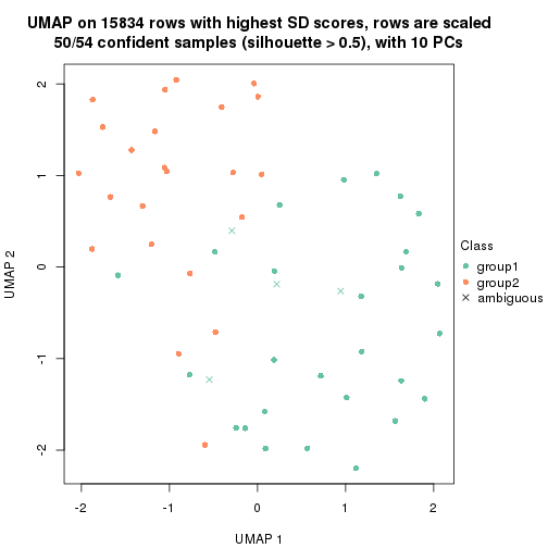
dimension_reduction(res, k = 3, method = "UMAP")
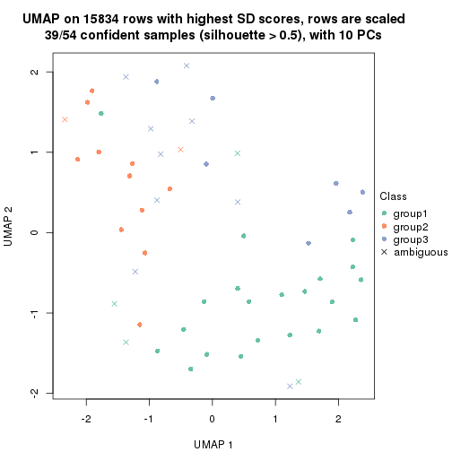
dimension_reduction(res, k = 4, method = "UMAP")
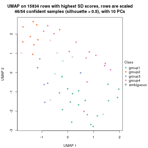
dimension_reduction(res, k = 5, method = "UMAP")
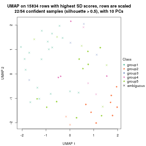
dimension_reduction(res, k = 6, method = "UMAP")
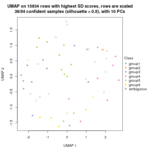
Following heatmap shows how subgroups are split when increasing k:
collect_classes(res)
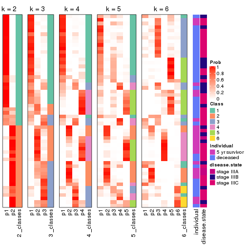
Test correlation between subgroups and known annotations. If the known annotation is numeric, one-way ANOVA test is applied, and if the known annotation is discrete, chi-squared contingency table test is applied.
test_to_known_factors(res)
#>         n individual(p) disease.state(p) k
#> SD:NMF 50       0.00539           0.1356 2
#> SD:NMF 39       0.01998           0.4673 3
#> SD:NMF 46       0.01022           0.1545 4
#> SD:NMF 22       0.05060           0.1457 5
#> SD:NMF 36       0.00201           0.0534 6
If matrix rows can be associated to genes, consider to use functional_enrichment(res,
...) to perform function enrichment for the signature genes. See this vignette for more detailed explanations.
The object with results only for a single top-value method and a single partition method can be extracted as:
res = res_list["CV", "hclust"]
# you can also extract it by
# res = res_list["CV:hclust"]
A summary of res and all the functions that can be applied to it:
res
#> A 'ConsensusPartition' object with k = 2, 3, 4, 5, 6.
#>   On a matrix with 15834 rows and 54 columns.
#>   Top rows (1000, 2000, 3000, 4000, 5000) are extracted by 'CV' method.
#>   Subgroups are detected by 'hclust' method.
#>   Performed in total 1250 partitions by row resampling.
#>   Best k for subgroups seems to be 5.
#>
#> Following methods can be applied to this 'ConsensusPartition' object:
#>  [1] "cola_report"             "collect_classes"         "collect_plots"
#>  [4] "collect_stats"           "colnames"                "compare_signatures"
#>  [7] "consensus_heatmap"       "dimension_reduction"     "functional_enrichment"
#> [10] "get_anno_col"            "get_anno"                "get_classes"
#> [13] "get_consensus"           "get_matrix"              "get_membership"
#> [16] "get_param"               "get_signatures"          "get_stats"
#> [19] "is_best_k"               "is_stable_k"             "membership_heatmap"
#> [22] "ncol"                    "nrow"                    "plot_ecdf"
#> [25] "rownames"                "select_partition_number" "show"
#> [28] "suggest_best_k"          "test_to_known_factors"
collect_plots() function collects all the plots made from res for all k (number of partitions)
into one single page to provide an easy and fast comparison between different k.
collect_plots(res)
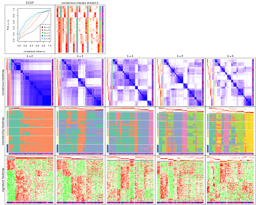
The plots are:
k and the heatmap of
predicted classes for each k.k.k.k.All the plots in panels can be made by individual functions and they are plotted later in this section.
select_partition_number() produces several plots showing different
statistics for choosing “optimized” k. There are following statistics:
k;k, the area increased is defined as \(A_k - A_{k-1}\).The detailed explanations of these statistics can be found in the cola vignette.
Generally speaking, lower PAC score, higher mean silhouette score or higher
concordance corresponds to better partition. Rand index and Jaccard index
measure how similar the current partition is compared to partition with k-1.
If they are too similar, we won't accept k is better than k-1.
select_partition_number(res)
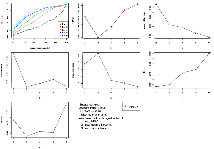
The numeric values for all these statistics can be obtained by get_stats().
get_stats(res)
#>   k 1-PAC mean_silhouette concordance area_increased  Rand Jaccard
#> 2 2 0.415           0.739       0.875         0.3860 0.628   0.628
#> 3 3 0.252           0.520       0.671         0.5299 0.647   0.471
#> 4 4 0.333           0.487       0.692         0.1463 0.763   0.519
#> 5 5 0.464           0.429       0.716         0.1055 0.795   0.506
#> 6 6 0.511           0.386       0.673         0.0531 0.947   0.781
suggest_best_k() suggests the best \(k\) based on these statistics. The rules are as follows:
suggest_best_k(res)
#> [1] 5
Following shows the table of the partitions (You need to click the show/hide
code output link to see it). The membership matrix (columns with name p*)
is inferred by
clue::cl_consensus()
function with the SE method. Basically the value in the membership matrix
represents the probability to belong to a certain group. The finall class
label for an item is determined with the group with highest probability it
belongs to.
In get_classes() function, the entropy is calculated from the membership
matrix and the silhouette score is calculated from the consensus matrix.
cbind(get_classes(res, k = 2), get_membership(res, k = 2))
#>           class entropy silhouette    p1    p2
#> GSM311939     2  0.0376     0.8591 0.004 0.996
#> GSM311963     2  0.7219     0.7365 0.200 0.800
#> GSM311973     1  0.8327     0.6478 0.736 0.264
#> GSM311940     2  0.2603     0.8655 0.044 0.956
#> GSM311953     2  0.2778     0.8653 0.048 0.952
#> GSM311974     2  0.2948     0.8649 0.052 0.948
#> GSM311975     2  0.5408     0.8279 0.124 0.876
#> GSM311977     2  0.2778     0.8654 0.048 0.952
#> GSM311982     1  0.0376     0.8017 0.996 0.004
#> GSM311990     2  0.0000     0.8606 0.000 1.000
#> GSM311943     2  0.8016     0.7090 0.244 0.756
#> GSM311944     2  0.9358     0.5063 0.352 0.648
#> GSM311946     2  0.2778     0.8653 0.048 0.952
#> GSM311956     1  0.6438     0.7529 0.836 0.164
#> GSM311967     2  0.0000     0.8606 0.000 1.000
#> GSM311968     2  0.4298     0.8522 0.088 0.912
#> GSM311972     1  0.0376     0.8017 0.996 0.004
#> GSM311980     1  0.6247     0.7572 0.844 0.156
#> GSM311981     1  0.0376     0.8017 0.996 0.004
#> GSM311988     2  0.0376     0.8591 0.004 0.996
#> GSM311957     2  0.2948     0.8640 0.052 0.948
#> GSM311960     2  0.4939     0.8439 0.108 0.892
#> GSM311971     1  0.9427     0.4532 0.640 0.360
#> GSM311976     2  0.9881     0.2140 0.436 0.564
#> GSM311978     1  0.4939     0.7682 0.892 0.108
#> GSM311979     1  0.0376     0.8017 0.996 0.004
#> GSM311983     2  0.7674     0.7341 0.224 0.776
#> GSM311986     2  0.0000     0.8606 0.000 1.000
#> GSM311991     1  0.0376     0.8017 0.996 0.004
#> GSM311938     2  0.1843     0.8653 0.028 0.972
#> GSM311941     2  0.1633     0.8660 0.024 0.976
#> GSM311942     2  0.3114     0.8621 0.056 0.944
#> GSM311945     2  0.4815     0.8455 0.104 0.896
#> GSM311947     2  0.0000     0.8606 0.000 1.000
#> GSM311948     2  0.2778     0.8658 0.048 0.952
#> GSM311949     2  0.9977     0.0827 0.472 0.528
#> GSM311950     2  0.0376     0.8591 0.004 0.996
#> GSM311951     2  0.3584     0.8594 0.068 0.932
#> GSM311952     2  0.8016     0.7090 0.244 0.756
#> GSM311954     2  0.0000     0.8606 0.000 1.000
#> GSM311955     2  0.7950     0.7131 0.240 0.760
#> GSM311958     2  0.8016     0.7078 0.244 0.756
#> GSM311959     2  0.0376     0.8604 0.004 0.996
#> GSM311961     2  0.2603     0.8626 0.044 0.956
#> GSM311962     1  0.9977     0.1186 0.528 0.472
#> GSM311964     2  0.9993     0.0345 0.484 0.516
#> GSM311965     2  0.6048     0.8149 0.148 0.852
#> GSM311966     1  0.9833     0.2877 0.576 0.424
#> GSM311969     2  0.0376     0.8604 0.004 0.996
#> GSM311970     1  0.0000     0.7992 1.000 0.000
#> GSM311984     2  0.0000     0.8606 0.000 1.000
#> GSM311985     2  0.9661     0.4191 0.392 0.608
#> GSM311987     2  0.0000     0.8606 0.000 1.000
#> GSM311989     2  0.4815     0.8455 0.104 0.896
cbind(get_classes(res, k = 3), get_membership(res, k = 3))
#>           class entropy silhouette    p1    p2    p3
#> GSM311939     3  0.2878     0.6850 0.096 0.000 0.904
#> GSM311963     3  0.9144     0.1161 0.408 0.144 0.448
#> GSM311973     2  0.7524     0.6048 0.180 0.692 0.128
#> GSM311940     3  0.6252     0.5385 0.344 0.008 0.648
#> GSM311953     3  0.6434     0.5038 0.380 0.008 0.612
#> GSM311974     3  0.6548     0.4942 0.372 0.012 0.616
#> GSM311975     3  0.7114     0.3136 0.388 0.028 0.584
#> GSM311977     3  0.6381     0.5372 0.340 0.012 0.648
#> GSM311982     2  0.5327     0.7318 0.272 0.728 0.000
#> GSM311990     3  0.0424     0.6895 0.008 0.000 0.992
#> GSM311943     1  0.5455     0.5984 0.788 0.028 0.184
#> GSM311944     1  0.7720     0.5391 0.672 0.120 0.208
#> GSM311946     3  0.6434     0.5038 0.380 0.008 0.612
#> GSM311956     2  0.5334     0.7255 0.060 0.820 0.120
#> GSM311967     3  0.0237     0.6891 0.004 0.000 0.996
#> GSM311968     1  0.6476     0.2630 0.548 0.004 0.448
#> GSM311972     2  0.5291     0.7339 0.268 0.732 0.000
#> GSM311980     2  0.5285     0.7310 0.064 0.824 0.112
#> GSM311981     2  0.0747     0.7849 0.016 0.984 0.000
#> GSM311988     3  0.4931     0.6266 0.232 0.000 0.768
#> GSM311957     1  0.6235     0.3212 0.564 0.000 0.436
#> GSM311960     1  0.6381     0.4600 0.648 0.012 0.340
#> GSM311971     1  0.7442     0.0362 0.588 0.368 0.044
#> GSM311976     1  0.8962     0.4686 0.548 0.288 0.164
#> GSM311978     2  0.6045     0.6012 0.380 0.620 0.000
#> GSM311979     2  0.5327     0.7318 0.272 0.728 0.000
#> GSM311983     1  0.5406     0.5911 0.780 0.020 0.200
#> GSM311986     3  0.0424     0.6895 0.008 0.000 0.992
#> GSM311991     2  0.0747     0.7849 0.016 0.984 0.000
#> GSM311938     3  0.5098     0.6275 0.248 0.000 0.752
#> GSM311941     3  0.4887     0.5882 0.228 0.000 0.772
#> GSM311942     1  0.6286     0.2224 0.536 0.000 0.464
#> GSM311945     1  0.6467     0.3751 0.604 0.008 0.388
#> GSM311947     3  0.0237     0.6891 0.004 0.000 0.996
#> GSM311948     3  0.6688     0.4166 0.408 0.012 0.580
#> GSM311949     1  0.9057     0.3997 0.520 0.324 0.156
#> GSM311950     3  0.1289     0.6938 0.032 0.000 0.968
#> GSM311951     1  0.6267     0.2500 0.548 0.000 0.452
#> GSM311952     1  0.5455     0.5984 0.788 0.028 0.184
#> GSM311954     3  0.0892     0.6908 0.020 0.000 0.980
#> GSM311955     1  0.5610     0.5962 0.776 0.028 0.196
#> GSM311958     1  0.5508     0.5955 0.784 0.028 0.188
#> GSM311959     3  0.2590     0.6537 0.072 0.004 0.924
#> GSM311961     1  0.6813     0.0361 0.520 0.012 0.468
#> GSM311962     1  0.7416     0.3026 0.656 0.276 0.068
#> GSM311964     1  0.9120     0.3700 0.504 0.340 0.156
#> GSM311965     1  0.7919     0.3907 0.556 0.064 0.380
#> GSM311966     1  0.7084     0.1973 0.652 0.304 0.044
#> GSM311969     3  0.2590     0.6537 0.072 0.004 0.924
#> GSM311970     2  0.0829     0.7850 0.012 0.984 0.004
#> GSM311984     3  0.6617     0.1648 0.436 0.008 0.556
#> GSM311985     1  0.7564     0.5491 0.692 0.156 0.152
#> GSM311987     3  0.0747     0.6890 0.016 0.000 0.984
#> GSM311989     1  0.6275     0.4574 0.644 0.008 0.348
cbind(get_classes(res, k = 4), get_membership(res, k = 4))
#>           class entropy silhouette    p1    p2    p3    p4
#> GSM311939     3   0.633     0.6532 0.168 0.052 0.712 0.068
#> GSM311963     1   0.907     0.2937 0.476 0.136 0.168 0.220
#> GSM311973     4   0.534     0.5592 0.152 0.024 0.056 0.768
#> GSM311940     1   0.765     0.0562 0.484 0.048 0.392 0.076
#> GSM311953     1   0.758     0.1520 0.512 0.032 0.356 0.100
#> GSM311974     1   0.752     0.1672 0.520 0.028 0.348 0.104
#> GSM311975     1   0.711     0.1333 0.484 0.112 0.400 0.004
#> GSM311977     1   0.771     0.0578 0.480 0.052 0.392 0.076
#> GSM311982     2   0.579     0.8898 0.060 0.656 0.000 0.284
#> GSM311990     3   0.112     0.8090 0.036 0.000 0.964 0.000
#> GSM311943     1   0.359     0.5190 0.824 0.168 0.008 0.000
#> GSM311944     1   0.559     0.4629 0.680 0.264 0.056 0.000
#> GSM311946     1   0.758     0.1520 0.512 0.032 0.356 0.100
#> GSM311956     4   0.229     0.7632 0.012 0.004 0.060 0.924
#> GSM311967     3   0.102     0.8081 0.032 0.000 0.968 0.000
#> GSM311968     1   0.453     0.5047 0.752 0.012 0.232 0.004
#> GSM311972     2   0.590     0.8946 0.068 0.652 0.000 0.280
#> GSM311980     4   0.240     0.7666 0.012 0.012 0.052 0.924
#> GSM311981     4   0.247     0.7626 0.000 0.108 0.000 0.892
#> GSM311988     3   0.838     0.2893 0.316 0.108 0.492 0.084
#> GSM311957     1   0.401     0.5357 0.800 0.016 0.184 0.000
#> GSM311960     1   0.380     0.5686 0.848 0.016 0.120 0.016
#> GSM311971     1   0.742    -0.2775 0.436 0.396 0.000 0.168
#> GSM311976     1   0.707     0.2607 0.620 0.160 0.016 0.204
#> GSM311978     2   0.612     0.7352 0.164 0.680 0.000 0.156
#> GSM311979     2   0.588     0.8959 0.068 0.656 0.000 0.276
#> GSM311983     1   0.354     0.5186 0.820 0.176 0.004 0.000
#> GSM311986     3   0.112     0.8090 0.036 0.000 0.964 0.000
#> GSM311991     4   0.247     0.7626 0.000 0.108 0.000 0.892
#> GSM311938     3   0.740     0.2477 0.360 0.044 0.528 0.068
#> GSM311941     3   0.468     0.4500 0.316 0.004 0.680 0.000
#> GSM311942     1   0.469     0.4903 0.732 0.012 0.252 0.004
#> GSM311945     1   0.429     0.5450 0.804 0.012 0.168 0.016
#> GSM311947     3   0.102     0.8081 0.032 0.000 0.968 0.000
#> GSM311948     1   0.713     0.2239 0.552 0.032 0.348 0.068
#> GSM311949     1   0.734     0.1649 0.580 0.156 0.016 0.248
#> GSM311950     3   0.380     0.7595 0.076 0.004 0.856 0.064
#> GSM311951     1   0.460     0.5006 0.744 0.012 0.240 0.004
#> GSM311952     1   0.359     0.5190 0.824 0.168 0.008 0.000
#> GSM311954     3   0.206     0.8070 0.052 0.016 0.932 0.000
#> GSM311955     1   0.395     0.5205 0.812 0.168 0.020 0.000
#> GSM311958     1   0.367     0.5082 0.808 0.188 0.004 0.000
#> GSM311959     3   0.277     0.7613 0.116 0.004 0.880 0.000
#> GSM311961     1   0.654     0.3949 0.604 0.284 0.112 0.000
#> GSM311962     1   0.678    -0.0149 0.528 0.368 0.000 0.104
#> GSM311964     1   0.740     0.1305 0.568 0.152 0.016 0.264
#> GSM311965     1   0.530     0.5453 0.752 0.080 0.164 0.004
#> GSM311966     1   0.686    -0.1286 0.488 0.408 0.000 0.104
#> GSM311969     3   0.277     0.7613 0.116 0.004 0.880 0.000
#> GSM311970     4   0.228     0.7687 0.000 0.096 0.000 0.904
#> GSM311984     1   0.739     0.2629 0.512 0.284 0.204 0.000
#> GSM311985     1   0.577     0.3869 0.632 0.332 0.020 0.016
#> GSM311987     3   0.139     0.8070 0.048 0.000 0.952 0.000
#> GSM311989     1   0.343     0.5672 0.860 0.012 0.120 0.008
cbind(get_classes(res, k = 5), get_membership(res, k = 5))
#>           class entropy silhouette    p1    p2    p3    p4    p5
#> GSM311939     3  0.5094    0.34016 0.000 0.352 0.600 0.000 0.048
#> GSM311963     2  0.6173    0.26687 0.180 0.664 0.004 0.068 0.084
#> GSM311973     4  0.6686    0.61580 0.128 0.152 0.000 0.620 0.100
#> GSM311940     2  0.7598    0.46230 0.048 0.392 0.252 0.000 0.308
#> GSM311953     2  0.7684    0.48070 0.052 0.392 0.208 0.004 0.344
#> GSM311974     5  0.7369   -0.42180 0.020 0.316 0.236 0.008 0.420
#> GSM311975     3  0.8287   -0.19669 0.200 0.136 0.396 0.004 0.264
#> GSM311977     2  0.7643    0.46283 0.052 0.392 0.252 0.000 0.304
#> GSM311982     1  0.3551    0.54294 0.772 0.000 0.000 0.220 0.008
#> GSM311990     3  0.0290    0.73107 0.000 0.000 0.992 0.000 0.008
#> GSM311943     5  0.4777    0.47029 0.268 0.052 0.000 0.000 0.680
#> GSM311944     5  0.4513    0.44938 0.284 0.004 0.024 0.000 0.688
#> GSM311946     2  0.7684    0.48070 0.052 0.392 0.208 0.004 0.344
#> GSM311956     4  0.3587    0.81847 0.012 0.152 0.004 0.820 0.012
#> GSM311967     3  0.0162    0.72870 0.000 0.000 0.996 0.000 0.004
#> GSM311968     5  0.3265    0.48740 0.020 0.012 0.120 0.000 0.848
#> GSM311972     1  0.3163    0.60502 0.824 0.000 0.000 0.164 0.012
#> GSM311980     4  0.3584    0.81886 0.020 0.148 0.000 0.820 0.012
#> GSM311981     4  0.0833    0.82769 0.016 0.004 0.000 0.976 0.004
#> GSM311988     2  0.5580    0.10206 0.012 0.604 0.320 0.000 0.064
#> GSM311957     5  0.3518    0.48962 0.008 0.048 0.104 0.000 0.840
#> GSM311960     5  0.1299    0.53740 0.008 0.012 0.020 0.000 0.960
#> GSM311971     1  0.5543    0.46232 0.612 0.016 0.000 0.056 0.316
#> GSM311976     5  0.6971    0.05182 0.312 0.056 0.000 0.120 0.512
#> GSM311978     1  0.1568    0.62395 0.944 0.000 0.000 0.036 0.020
#> GSM311979     1  0.3081    0.61069 0.832 0.000 0.000 0.156 0.012
#> GSM311983     5  0.5700    0.41312 0.280 0.120 0.000 0.000 0.600
#> GSM311986     3  0.0290    0.73107 0.000 0.000 0.992 0.000 0.008
#> GSM311991     4  0.0833    0.82769 0.016 0.004 0.000 0.976 0.004
#> GSM311938     3  0.7294   -0.31600 0.032 0.364 0.392 0.000 0.212
#> GSM311941     3  0.4252    0.30326 0.000 0.008 0.652 0.000 0.340
#> GSM311942     5  0.2806    0.47826 0.004 0.000 0.152 0.000 0.844
#> GSM311945     5  0.2102    0.52116 0.004 0.012 0.068 0.000 0.916
#> GSM311947     3  0.0290    0.72872 0.000 0.000 0.992 0.000 0.008
#> GSM311948     5  0.7549   -0.36483 0.040 0.272 0.252 0.004 0.432
#> GSM311949     5  0.7151    0.02007 0.264 0.052 0.000 0.172 0.512
#> GSM311950     3  0.3663    0.54051 0.000 0.208 0.776 0.000 0.016
#> GSM311951     5  0.2674    0.48439 0.004 0.000 0.140 0.000 0.856
#> GSM311952     5  0.4777    0.47029 0.268 0.052 0.000 0.000 0.680
#> GSM311954     3  0.1195    0.72775 0.000 0.028 0.960 0.000 0.012
#> GSM311955     5  0.5152    0.46699 0.268 0.052 0.012 0.000 0.668
#> GSM311958     5  0.5252    0.42944 0.292 0.076 0.000 0.000 0.632
#> GSM311959     3  0.2177    0.69068 0.004 0.008 0.908 0.000 0.080
#> GSM311961     2  0.5033   -0.18160 0.024 0.524 0.000 0.004 0.448
#> GSM311962     1  0.4935    0.35381 0.616 0.040 0.000 0.000 0.344
#> GSM311964     5  0.7209    0.02301 0.228 0.052 0.000 0.208 0.512
#> GSM311965     5  0.3180    0.51325 0.076 0.000 0.068 0.000 0.856
#> GSM311966     1  0.4503    0.42470 0.664 0.024 0.000 0.000 0.312
#> GSM311969     3  0.2177    0.69068 0.004 0.008 0.908 0.000 0.080
#> GSM311970     4  0.0693    0.83171 0.012 0.008 0.000 0.980 0.000
#> GSM311984     2  0.6229   -0.00255 0.008 0.524 0.104 0.004 0.360
#> GSM311985     5  0.5485    0.22309 0.452 0.044 0.008 0.000 0.496
#> GSM311987     3  0.0693    0.72899 0.000 0.008 0.980 0.000 0.012
#> GSM311989     5  0.0932    0.53947 0.004 0.004 0.020 0.000 0.972
cbind(get_classes(res, k = 6), get_membership(res, k = 6))
#>           class entropy silhouette    p1    p2    p3    p4    p5    p6
#> GSM311939     6  0.5765     0.2638 0.004 0.288 0.128 0.000 0.016 0.564
#> GSM311963     2  0.3954     0.3137 0.104 0.812 0.020 0.044 0.016 0.004
#> GSM311973     4  0.4968     0.6075 0.080 0.108 0.000 0.724 0.088 0.000
#> GSM311940     2  0.6094     0.6711 0.008 0.524 0.000 0.008 0.228 0.232
#> GSM311953     2  0.7213     0.6205 0.012 0.448 0.000 0.088 0.264 0.188
#> GSM311974     5  0.7670    -0.4083 0.012 0.252 0.000 0.140 0.380 0.216
#> GSM311975     6  0.8033    -0.2121 0.136 0.224 0.036 0.004 0.204 0.396
#> GSM311977     2  0.6183     0.6710 0.012 0.520 0.000 0.008 0.228 0.232
#> GSM311982     1  0.3103     0.4752 0.784 0.000 0.000 0.208 0.008 0.000
#> GSM311990     6  0.0405     0.7572 0.000 0.004 0.000 0.000 0.008 0.988
#> GSM311943     5  0.7094    -0.2565 0.212 0.076 0.292 0.000 0.416 0.004
#> GSM311944     5  0.6294    -0.0591 0.276 0.004 0.204 0.000 0.496 0.020
#> GSM311946     2  0.7213     0.6205 0.012 0.448 0.000 0.088 0.264 0.188
#> GSM311956     4  0.1080     0.8105 0.000 0.032 0.000 0.960 0.004 0.004
#> GSM311967     6  0.0748     0.7511 0.000 0.016 0.004 0.000 0.004 0.976
#> GSM311968     5  0.3335     0.4421 0.012 0.040 0.000 0.012 0.844 0.092
#> GSM311972     1  0.3192     0.5695 0.848 0.032 0.008 0.100 0.012 0.000
#> GSM311980     4  0.1116     0.8104 0.004 0.028 0.000 0.960 0.008 0.000
#> GSM311981     4  0.4077     0.7902 0.008 0.044 0.212 0.736 0.000 0.000
#> GSM311988     2  0.4626     0.3144 0.008 0.672 0.020 0.000 0.024 0.276
#> GSM311957     5  0.3292     0.4028 0.008 0.056 0.008 0.000 0.844 0.084
#> GSM311960     5  0.0810     0.4422 0.008 0.004 0.000 0.008 0.976 0.004
#> GSM311971     1  0.5401     0.4763 0.604 0.068 0.016 0.012 0.300 0.000
#> GSM311976     5  0.7273    -0.0742 0.288 0.156 0.028 0.076 0.452 0.000
#> GSM311978     1  0.1448     0.5499 0.948 0.024 0.000 0.016 0.012 0.000
#> GSM311979     1  0.2841     0.5716 0.864 0.032 0.000 0.092 0.012 0.000
#> GSM311983     3  0.7395     0.1429 0.208 0.132 0.344 0.000 0.316 0.000
#> GSM311986     6  0.0405     0.7572 0.000 0.004 0.000 0.000 0.008 0.988
#> GSM311991     4  0.4077     0.7902 0.008 0.044 0.212 0.736 0.000 0.000
#> GSM311938     2  0.5557     0.4915 0.004 0.512 0.000 0.000 0.128 0.356
#> GSM311941     6  0.3819     0.2913 0.000 0.000 0.008 0.000 0.340 0.652
#> GSM311942     5  0.2320     0.4387 0.000 0.004 0.000 0.000 0.864 0.132
#> GSM311945     5  0.1686     0.4501 0.004 0.004 0.000 0.008 0.932 0.052
#> GSM311947     6  0.0951     0.7503 0.000 0.020 0.004 0.000 0.008 0.968
#> GSM311948     5  0.7417    -0.3795 0.012 0.272 0.000 0.088 0.392 0.236
#> GSM311949     5  0.7477    -0.0874 0.260 0.132 0.028 0.128 0.452 0.000
#> GSM311950     6  0.3354     0.4980 0.000 0.240 0.004 0.000 0.004 0.752
#> GSM311951     5  0.2191     0.4425 0.000 0.004 0.000 0.000 0.876 0.120
#> GSM311952     5  0.7094    -0.2565 0.212 0.076 0.292 0.000 0.416 0.004
#> GSM311954     6  0.1659     0.7492 0.004 0.028 0.020 0.000 0.008 0.940
#> GSM311955     5  0.7270    -0.2615 0.212 0.068 0.292 0.000 0.412 0.016
#> GSM311958     5  0.7466    -0.3455 0.220 0.120 0.296 0.000 0.360 0.004
#> GSM311959     6  0.2341     0.7221 0.000 0.012 0.032 0.000 0.056 0.900
#> GSM311961     3  0.3621     0.5688 0.004 0.032 0.772 0.000 0.192 0.000
#> GSM311962     1  0.5414     0.4161 0.580 0.072 0.028 0.000 0.320 0.000
#> GSM311964     5  0.7553    -0.0764 0.228 0.120 0.028 0.172 0.452 0.000
#> GSM311965     5  0.3920     0.4020 0.064 0.004 0.072 0.000 0.812 0.048
#> GSM311966     1  0.5107     0.4558 0.620 0.060 0.024 0.000 0.296 0.000
#> GSM311969     6  0.2341     0.7221 0.000 0.012 0.032 0.000 0.056 0.900
#> GSM311970     4  0.2389     0.8136 0.000 0.008 0.128 0.864 0.000 0.000
#> GSM311984     3  0.5044     0.5292 0.000 0.036 0.696 0.000 0.164 0.104
#> GSM311985     1  0.7466    -0.2959 0.384 0.108 0.228 0.000 0.272 0.008
#> GSM311987     6  0.0520     0.7566 0.000 0.000 0.008 0.000 0.008 0.984
#> GSM311989     5  0.0436     0.4408 0.004 0.004 0.000 0.000 0.988 0.004
Heatmaps for the consensus matrix. It visualizes the probability of two samples to be in a same group.
consensus_heatmap(res, k = 2)
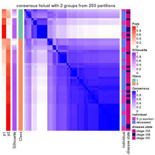
consensus_heatmap(res, k = 3)
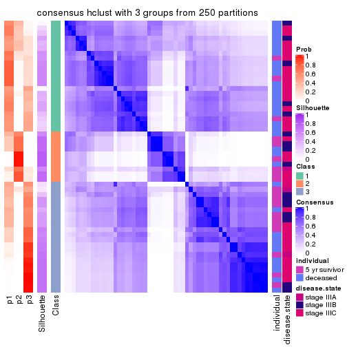
consensus_heatmap(res, k = 4)
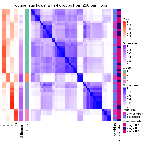
consensus_heatmap(res, k = 5)
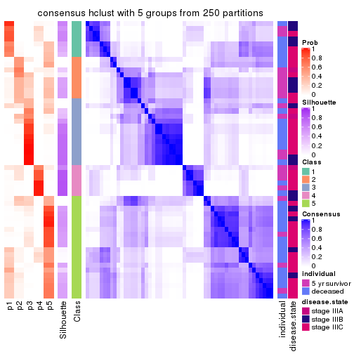
consensus_heatmap(res, k = 6)
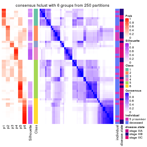
Heatmaps for the membership of samples in all partitions to see how consistent they are:
membership_heatmap(res, k = 2)
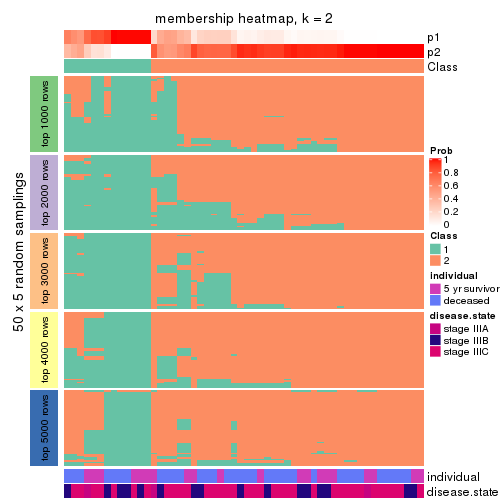
membership_heatmap(res, k = 3)
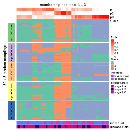
membership_heatmap(res, k = 4)
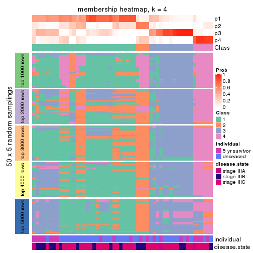
membership_heatmap(res, k = 5)
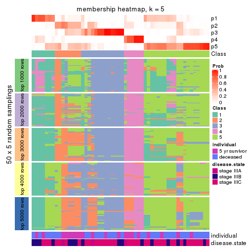
membership_heatmap(res, k = 6)
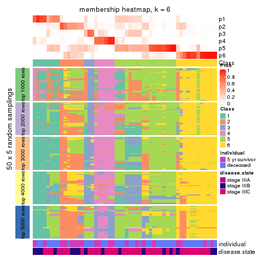
As soon as we have had the classes for columns, we can look for signatures which are significantly different between classes which can be candidate marks for certain classes. Following are the heatmaps for signatures.
Signature heatmaps where rows are scaled:
get_signatures(res, k = 2)
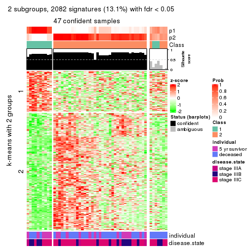
get_signatures(res, k = 3)
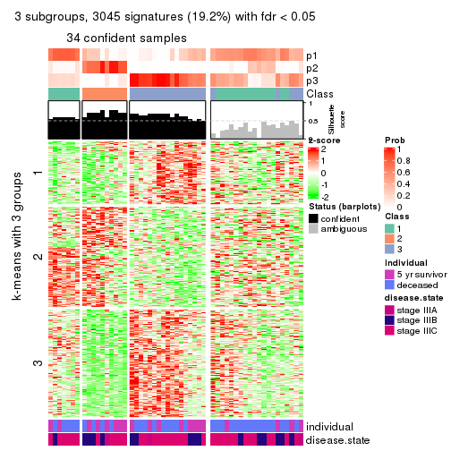
get_signatures(res, k = 4)
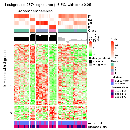
get_signatures(res, k = 5)
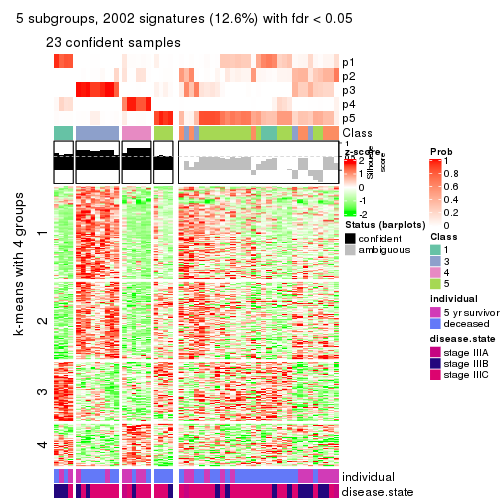
get_signatures(res, k = 6)
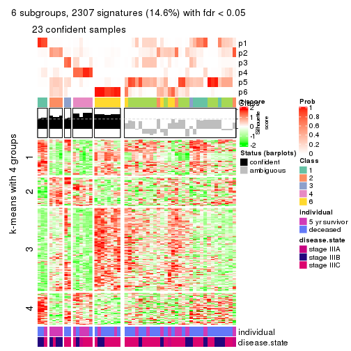
Signature heatmaps where rows are not scaled:
get_signatures(res, k = 2, scale_rows = FALSE)
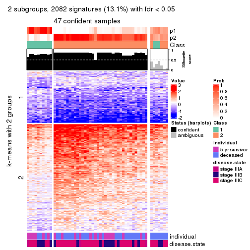
get_signatures(res, k = 3, scale_rows = FALSE)
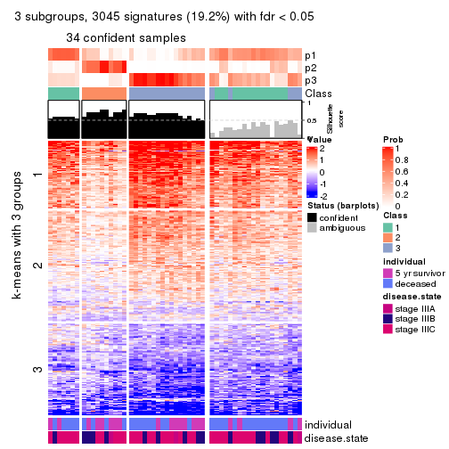
get_signatures(res, k = 4, scale_rows = FALSE)
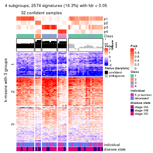
get_signatures(res, k = 5, scale_rows = FALSE)
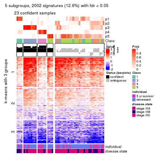
get_signatures(res, k = 6, scale_rows = FALSE)
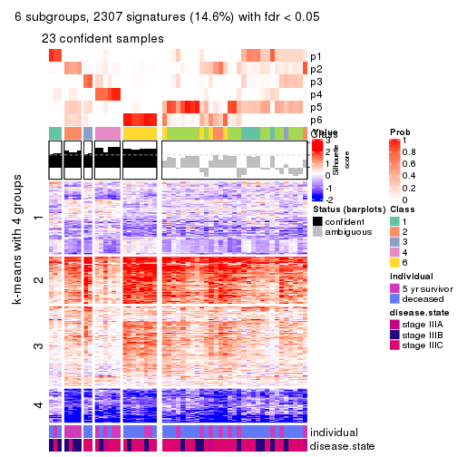
Compare the overlap of signatures from different k:
compare_signatures(res)
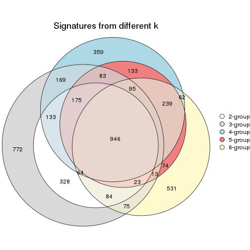
get_signature() returns a data frame invisibly. TO get the list of signatures, the function
call should be assigned to a variable explicitly. In following code, if plot argument is set
to FALSE, no heatmap is plotted while only the differential analysis is performed.
# code only for demonstration
tb = get_signature(res, k = ..., plot = FALSE)
An example of the output of tb is:
#>   which_row         fdr    mean_1    mean_2 scaled_mean_1 scaled_mean_2 km
#> 1        38 0.042760348  8.373488  9.131774    -0.5533452     0.5164555  1
#> 2        40 0.018707592  7.106213  8.469186    -0.6173731     0.5762149  1
#> 3        55 0.019134737 10.221463 11.207825    -0.6159697     0.5749050  1
#> 4        59 0.006059896  5.921854  7.869574    -0.6899429     0.6439467  1
#> 5        60 0.018055526  8.928898 10.211722    -0.6204761     0.5791110  1
#> 6        98 0.009384629 15.714769 14.887706     0.6635654    -0.6193277  2
...
The columns in tb are:
which_row: row indices corresponding to the input matrix.fdr: FDR for the differential test. mean_x: The mean value in group x.scaled_mean_x: The mean value in group x after rows are scaled.km: Row groups if k-means clustering is applied to rows.UMAP plot which shows how samples are separated.
dimension_reduction(res, k = 2, method = "UMAP")
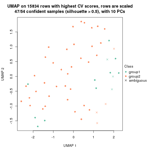
dimension_reduction(res, k = 3, method = "UMAP")
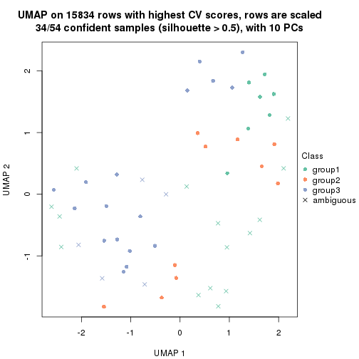
dimension_reduction(res, k = 4, method = "UMAP")
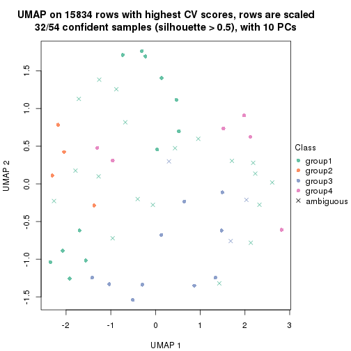
dimension_reduction(res, k = 5, method = "UMAP")
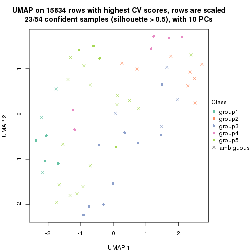
dimension_reduction(res, k = 6, method = "UMAP")
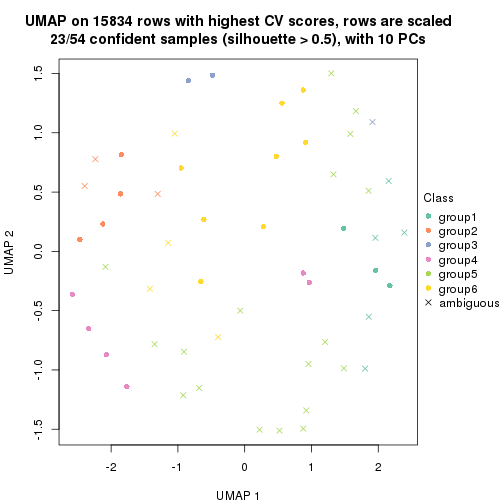
Following heatmap shows how subgroups are split when increasing k:
collect_classes(res)
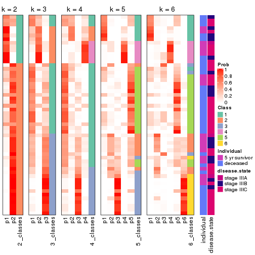
Test correlation between subgroups and known annotations. If the known annotation is numeric, one-way ANOVA test is applied, and if the known annotation is discrete, chi-squared contingency table test is applied.
test_to_known_factors(res)
#>            n individual(p) disease.state(p) k
#> CV:hclust 47        0.3696            0.581 2
#> CV:hclust 34        0.4421            0.656 3
#> CV:hclust 32        0.1748            0.308 4
#> CV:hclust 23        0.1188            0.292 5
#> CV:hclust 23        0.0618            0.336 6
If matrix rows can be associated to genes, consider to use functional_enrichment(res,
...) to perform function enrichment for the signature genes. See this vignette for more detailed explanations.
The object with results only for a single top-value method and a single partition method can be extracted as:
res = res_list["CV", "kmeans"]
# you can also extract it by
# res = res_list["CV:kmeans"]
A summary of res and all the functions that can be applied to it:
res
#> A 'ConsensusPartition' object with k = 2, 3, 4, 5, 6.
#>   On a matrix with 15834 rows and 54 columns.
#>   Top rows (1000, 2000, 3000, 4000, 5000) are extracted by 'CV' method.
#>   Subgroups are detected by 'kmeans' method.
#>   Performed in total 1250 partitions by row resampling.
#>   Best k for subgroups seems to be 2.
#>
#> Following methods can be applied to this 'ConsensusPartition' object:
#>  [1] "cola_report"             "collect_classes"         "collect_plots"
#>  [4] "collect_stats"           "colnames"                "compare_signatures"
#>  [7] "consensus_heatmap"       "dimension_reduction"     "functional_enrichment"
#> [10] "get_anno_col"            "get_anno"                "get_classes"
#> [13] "get_consensus"           "get_matrix"              "get_membership"
#> [16] "get_param"               "get_signatures"          "get_stats"
#> [19] "is_best_k"               "is_stable_k"             "membership_heatmap"
#> [22] "ncol"                    "nrow"                    "plot_ecdf"
#> [25] "rownames"                "select_partition_number" "show"
#> [28] "suggest_best_k"          "test_to_known_factors"
collect_plots() function collects all the plots made from res for all k (number of partitions)
into one single page to provide an easy and fast comparison between different k.
collect_plots(res)
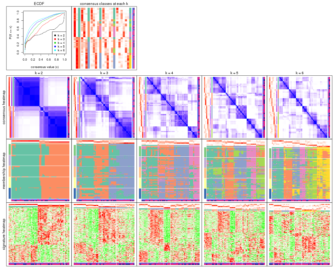
The plots are:
k and the heatmap of
predicted classes for each k.k.k.k.All the plots in panels can be made by individual functions and they are plotted later in this section.
select_partition_number() produces several plots showing different
statistics for choosing “optimized” k. There are following statistics:
k;k, the area increased is defined as \(A_k - A_{k-1}\).The detailed explanations of these statistics can be found in the cola vignette.
Generally speaking, lower PAC score, higher mean silhouette score or higher
concordance corresponds to better partition. Rand index and Jaccard index
measure how similar the current partition is compared to partition with k-1.
If they are too similar, we won't accept k is better than k-1.
select_partition_number(res)

The numeric values for all these statistics can be obtained by get_stats().
get_stats(res)
#>   k 1-PAC mean_silhouette concordance area_increased  Rand Jaccard
#> 2 2 0.656           0.854       0.929         0.5040 0.491   0.491
#> 3 3 0.389           0.510       0.715         0.2998 0.782   0.585
#> 4 4 0.403           0.482       0.676         0.1310 0.787   0.464
#> 5 5 0.507           0.476       0.631         0.0699 0.905   0.641
#> 6 6 0.591           0.539       0.663         0.0422 0.899   0.558
suggest_best_k() suggests the best \(k\) based on these statistics. The rules are as follows:
suggest_best_k(res)
#> [1] 2
Following shows the table of the partitions (You need to click the show/hide
code output link to see it). The membership matrix (columns with name p*)
is inferred by
clue::cl_consensus()
function with the SE method. Basically the value in the membership matrix
represents the probability to belong to a certain group. The finall class
label for an item is determined with the group with highest probability it
belongs to.
In get_classes() function, the entropy is calculated from the membership
matrix and the silhouette score is calculated from the consensus matrix.
cbind(get_classes(res, k = 2), get_membership(res, k = 2))
#>           class entropy silhouette    p1    p2
#> GSM311939     2  0.0000      0.887 0.000 1.000
#> GSM311963     2  0.9954      0.293 0.460 0.540
#> GSM311973     1  0.0376      0.957 0.996 0.004
#> GSM311940     2  0.6438      0.796 0.164 0.836
#> GSM311953     2  0.7376      0.754 0.208 0.792
#> GSM311974     2  0.6712      0.785 0.176 0.824
#> GSM311975     1  0.5737      0.826 0.864 0.136
#> GSM311977     2  0.9608      0.481 0.384 0.616
#> GSM311982     1  0.1184      0.957 0.984 0.016
#> GSM311990     2  0.0000      0.887 0.000 1.000
#> GSM311943     2  0.7815      0.667 0.232 0.768
#> GSM311944     1  0.7950      0.688 0.760 0.240
#> GSM311946     2  0.9881      0.361 0.436 0.564
#> GSM311956     1  0.1414      0.949 0.980 0.020
#> GSM311967     2  0.1184      0.884 0.016 0.984
#> GSM311968     2  0.0938      0.885 0.012 0.988
#> GSM311972     1  0.0672      0.958 0.992 0.008
#> GSM311980     1  0.0376      0.957 0.996 0.004
#> GSM311981     1  0.0000      0.958 1.000 0.000
#> GSM311988     2  0.1184      0.884 0.016 0.984
#> GSM311957     2  0.0000      0.887 0.000 1.000
#> GSM311960     1  0.0376      0.957 0.996 0.004
#> GSM311971     1  0.1184      0.957 0.984 0.016
#> GSM311976     1  0.0000      0.958 1.000 0.000
#> GSM311978     1  0.1184      0.957 0.984 0.016
#> GSM311979     1  0.1184      0.957 0.984 0.016
#> GSM311983     1  0.5519      0.866 0.872 0.128
#> GSM311986     2  0.0000      0.887 0.000 1.000
#> GSM311991     1  0.0000      0.958 1.000 0.000
#> GSM311938     2  0.1184      0.884 0.016 0.984
#> GSM311941     2  0.0000      0.887 0.000 1.000
#> GSM311942     2  0.0000      0.887 0.000 1.000
#> GSM311945     1  0.0376      0.957 0.996 0.004
#> GSM311947     2  0.1184      0.884 0.016 0.984
#> GSM311948     2  0.6623      0.789 0.172 0.828
#> GSM311949     1  0.0000      0.958 1.000 0.000
#> GSM311950     2  0.1184      0.884 0.016 0.984
#> GSM311951     2  0.0000      0.887 0.000 1.000
#> GSM311952     1  0.2423      0.948 0.960 0.040
#> GSM311954     2  0.0000      0.887 0.000 1.000
#> GSM311955     1  0.5842      0.850 0.860 0.140
#> GSM311958     1  0.2423      0.948 0.960 0.040
#> GSM311959     2  0.1843      0.877 0.028 0.972
#> GSM311961     2  0.9977      0.171 0.472 0.528
#> GSM311962     1  0.2423      0.948 0.960 0.040
#> GSM311964     1  0.0000      0.958 1.000 0.000
#> GSM311965     2  0.0938      0.885 0.012 0.988
#> GSM311966     1  0.1184      0.957 0.984 0.016
#> GSM311969     2  0.1843      0.877 0.028 0.972
#> GSM311970     1  0.0376      0.957 0.996 0.004
#> GSM311984     2  0.0000      0.887 0.000 1.000
#> GSM311985     1  0.1184      0.957 0.984 0.016
#> GSM311987     2  0.0000      0.887 0.000 1.000
#> GSM311989     1  0.3584      0.924 0.932 0.068
cbind(get_classes(res, k = 3), get_membership(res, k = 3))
#>           class entropy silhouette    p1    p2    p3
#> GSM311939     3  0.2682     0.6997 0.076 0.004 0.920
#> GSM311963     3  0.9967     0.0840 0.324 0.304 0.372
#> GSM311973     2  0.5070     0.5070 0.224 0.772 0.004
#> GSM311940     3  0.9405     0.3425 0.260 0.232 0.508
#> GSM311953     3  0.9777     0.2232 0.324 0.248 0.428
#> GSM311974     3  0.9842     0.2111 0.328 0.260 0.412
#> GSM311975     1  0.7344     0.4986 0.696 0.100 0.204
#> GSM311977     3  0.9862     0.1398 0.352 0.256 0.392
#> GSM311982     2  0.6079     0.5828 0.388 0.612 0.000
#> GSM311990     3  0.2066     0.6992 0.060 0.000 0.940
#> GSM311943     1  0.3816     0.5850 0.852 0.000 0.148
#> GSM311944     1  0.3112     0.6822 0.916 0.056 0.028
#> GSM311946     1  0.9949    -0.1772 0.360 0.284 0.356
#> GSM311956     2  0.1129     0.6281 0.004 0.976 0.020
#> GSM311967     3  0.0661     0.6947 0.004 0.008 0.988
#> GSM311968     3  0.7671     0.4796 0.380 0.052 0.568
#> GSM311972     2  0.6062     0.5830 0.384 0.616 0.000
#> GSM311980     2  0.0829     0.6471 0.012 0.984 0.004
#> GSM311981     2  0.4178     0.6790 0.172 0.828 0.000
#> GSM311988     3  0.1129     0.6933 0.020 0.004 0.976
#> GSM311957     1  0.6416    -0.0742 0.616 0.008 0.376
#> GSM311960     2  0.3896     0.6491 0.128 0.864 0.008
#> GSM311971     1  0.6180    -0.2637 0.584 0.416 0.000
#> GSM311976     2  0.6305     0.4236 0.484 0.516 0.000
#> GSM311978     1  0.6302    -0.4288 0.520 0.480 0.000
#> GSM311979     2  0.6095     0.5789 0.392 0.608 0.000
#> GSM311983     1  0.0829     0.7010 0.984 0.012 0.004
#> GSM311986     3  0.2711     0.6951 0.088 0.000 0.912
#> GSM311991     2  0.4346     0.6770 0.184 0.816 0.000
#> GSM311938     3  0.5378     0.5844 0.236 0.008 0.756
#> GSM311941     3  0.4399     0.6484 0.188 0.000 0.812
#> GSM311942     3  0.5951     0.6356 0.196 0.040 0.764
#> GSM311945     2  0.6513     0.2023 0.400 0.592 0.008
#> GSM311947     3  0.1585     0.6920 0.008 0.028 0.964
#> GSM311948     3  0.8967     0.2930 0.380 0.132 0.488
#> GSM311949     2  0.6308     0.4059 0.492 0.508 0.000
#> GSM311950     3  0.0424     0.6929 0.000 0.008 0.992
#> GSM311951     3  0.7328     0.5053 0.364 0.040 0.596
#> GSM311952     1  0.1647     0.6989 0.960 0.036 0.004
#> GSM311954     3  0.2959     0.6971 0.100 0.000 0.900
#> GSM311955     1  0.1337     0.7012 0.972 0.016 0.012
#> GSM311958     1  0.1647     0.6989 0.960 0.036 0.004
#> GSM311959     3  0.5327     0.5813 0.272 0.000 0.728
#> GSM311961     1  0.2165     0.6718 0.936 0.000 0.064
#> GSM311962     1  0.1267     0.7015 0.972 0.024 0.004
#> GSM311964     2  0.5591     0.6456 0.304 0.696 0.000
#> GSM311965     3  0.7794     0.4821 0.368 0.060 0.572
#> GSM311966     1  0.2878     0.6427 0.904 0.096 0.000
#> GSM311969     3  0.5397     0.5763 0.280 0.000 0.720
#> GSM311970     2  0.0829     0.6471 0.012 0.984 0.004
#> GSM311984     3  0.2711     0.6992 0.088 0.000 0.912
#> GSM311985     1  0.2959     0.6395 0.900 0.100 0.000
#> GSM311987     3  0.2537     0.6966 0.080 0.000 0.920
#> GSM311989     1  0.3370     0.6766 0.904 0.072 0.024
cbind(get_classes(res, k = 4), get_membership(res, k = 4))
#>           class entropy silhouette    p1    p2    p3    p4
#> GSM311939     3   0.361     0.7089 0.032 0.096 0.864 0.008
#> GSM311963     2   0.954     0.2760 0.240 0.324 0.320 0.116
#> GSM311973     4   0.722     0.2168 0.152 0.348 0.000 0.500
#> GSM311940     2   0.777     0.4286 0.064 0.524 0.336 0.076
#> GSM311953     2   0.780     0.4652 0.072 0.540 0.312 0.076
#> GSM311974     2   0.691     0.5148 0.048 0.640 0.244 0.068
#> GSM311975     1   0.771     0.2819 0.552 0.248 0.176 0.024
#> GSM311977     2   0.851     0.4432 0.120 0.488 0.304 0.088
#> GSM311982     4   0.612     0.4016 0.436 0.048 0.000 0.516
#> GSM311990     3   0.292     0.7121 0.000 0.140 0.860 0.000
#> GSM311943     1   0.700     0.3064 0.520 0.368 0.108 0.004
#> GSM311944     1   0.602     0.1774 0.488 0.480 0.016 0.016
#> GSM311946     2   0.823     0.4878 0.116 0.540 0.260 0.084
#> GSM311956     4   0.303     0.6048 0.000 0.124 0.008 0.868
#> GSM311967     3   0.213     0.7145 0.000 0.076 0.920 0.004
#> GSM311968     2   0.502     0.4553 0.044 0.736 0.220 0.000
#> GSM311972     4   0.534     0.4430 0.424 0.012 0.000 0.564
#> GSM311980     4   0.240     0.6431 0.004 0.092 0.000 0.904
#> GSM311981     4   0.253     0.6628 0.112 0.000 0.000 0.888
#> GSM311988     3   0.371     0.6368 0.000 0.148 0.832 0.020
#> GSM311957     2   0.700     0.3311 0.208 0.632 0.140 0.020
#> GSM311960     2   0.607    -0.1644 0.044 0.504 0.000 0.452
#> GSM311971     1   0.565     0.3137 0.708 0.088 0.000 0.204
#> GSM311976     1   0.678     0.0998 0.560 0.116 0.000 0.324
#> GSM311978     1   0.496     0.2977 0.732 0.036 0.000 0.232
#> GSM311979     4   0.614     0.3828 0.452 0.048 0.000 0.500
#> GSM311983     1   0.357     0.6355 0.848 0.132 0.016 0.004
#> GSM311986     3   0.325     0.7340 0.060 0.060 0.880 0.000
#> GSM311991     4   0.253     0.6628 0.112 0.000 0.000 0.888
#> GSM311938     3   0.685     0.3484 0.112 0.232 0.636 0.020
#> GSM311941     3   0.464     0.6429 0.040 0.188 0.772 0.000
#> GSM311942     2   0.558     0.2559 0.032 0.620 0.348 0.000
#> GSM311945     2   0.553     0.3803 0.092 0.736 0.004 0.168
#> GSM311947     3   0.409     0.5853 0.000 0.232 0.764 0.004
#> GSM311948     2   0.518     0.5479 0.060 0.760 0.172 0.008
#> GSM311949     1   0.687     0.0869 0.544 0.120 0.000 0.336
#> GSM311950     3   0.255     0.6997 0.000 0.092 0.900 0.008
#> GSM311951     2   0.502     0.4557 0.036 0.724 0.240 0.000
#> GSM311952     1   0.442     0.6184 0.784 0.192 0.016 0.008
#> GSM311954     3   0.376     0.7393 0.072 0.076 0.852 0.000
#> GSM311955     1   0.557     0.5273 0.676 0.280 0.040 0.004
#> GSM311958     1   0.438     0.6199 0.788 0.188 0.016 0.008
#> GSM311959     3   0.657     0.5270 0.184 0.164 0.648 0.004
#> GSM311961     1   0.678     0.5364 0.672 0.188 0.100 0.040
#> GSM311962     1   0.272     0.6253 0.908 0.068 0.012 0.012
#> GSM311964     4   0.549     0.5600 0.296 0.040 0.000 0.664
#> GSM311965     2   0.507     0.4571 0.040 0.724 0.236 0.000
#> GSM311966     1   0.247     0.5691 0.916 0.028 0.000 0.056
#> GSM311969     3   0.688     0.4932 0.216 0.168 0.612 0.004
#> GSM311970     4   0.198     0.6553 0.016 0.048 0.000 0.936
#> GSM311984     3   0.357     0.7344 0.068 0.052 0.872 0.008
#> GSM311985     1   0.304     0.5577 0.888 0.036 0.000 0.076
#> GSM311987     3   0.275     0.7446 0.056 0.040 0.904 0.000
#> GSM311989     2   0.517     0.1706 0.284 0.692 0.016 0.008
cbind(get_classes(res, k = 5), get_membership(res, k = 5))
#>           class entropy silhouette    p1    p2    p3    p4    p5
#> GSM311939     3  0.5284      0.556 0.012 0.244 0.680 0.004 0.060
#> GSM311963     2  0.5246      0.487 0.216 0.704 0.056 0.008 0.016
#> GSM311973     2  0.8147     -0.168 0.100 0.328 0.000 0.300 0.272
#> GSM311940     2  0.2852      0.560 0.012 0.892 0.064 0.008 0.024
#> GSM311953     2  0.2290      0.561 0.016 0.920 0.044 0.004 0.016
#> GSM311974     2  0.2424      0.513 0.004 0.908 0.024 0.004 0.060
#> GSM311975     1  0.7447      0.459 0.584 0.196 0.092 0.044 0.084
#> GSM311977     2  0.3105      0.570 0.088 0.864 0.044 0.004 0.000
#> GSM311982     4  0.6598      0.436 0.352 0.004 0.000 0.456 0.188
#> GSM311990     3  0.3950      0.675 0.000 0.068 0.796 0.000 0.136
#> GSM311943     1  0.7672      0.337 0.500 0.140 0.208 0.000 0.152
#> GSM311944     5  0.6404      0.471 0.264 0.168 0.012 0.000 0.556
#> GSM311946     2  0.2374      0.569 0.052 0.912 0.028 0.004 0.004
#> GSM311956     4  0.3002      0.570 0.000 0.116 0.000 0.856 0.028
#> GSM311967     3  0.5245      0.608 0.000 0.180 0.704 0.012 0.104
#> GSM311968     5  0.6713      0.654 0.012 0.256 0.180 0.008 0.544
#> GSM311972     4  0.6426      0.436 0.348 0.000 0.000 0.468 0.184
#> GSM311980     4  0.2735      0.596 0.000 0.084 0.000 0.880 0.036
#> GSM311981     4  0.3508      0.630 0.064 0.012 0.000 0.848 0.076
#> GSM311988     2  0.5459     -0.187 0.000 0.472 0.468 0.000 0.060
#> GSM311957     2  0.8222     -0.165 0.212 0.376 0.136 0.000 0.276
#> GSM311960     5  0.7399      0.244 0.028 0.292 0.000 0.312 0.368
#> GSM311971     1  0.6107      0.312 0.644 0.044 0.000 0.104 0.208
#> GSM311976     1  0.6553      0.354 0.624 0.072 0.000 0.168 0.136
#> GSM311978     1  0.5398      0.318 0.684 0.008 0.000 0.124 0.184
#> GSM311979     4  0.6532      0.390 0.384 0.000 0.000 0.420 0.196
#> GSM311983     1  0.4239      0.637 0.820 0.048 0.068 0.004 0.060
#> GSM311986     3  0.1413      0.732 0.012 0.020 0.956 0.000 0.012
#> GSM311991     4  0.3508      0.630 0.064 0.012 0.000 0.848 0.076
#> GSM311938     2  0.6266      0.152 0.040 0.568 0.332 0.008 0.052
#> GSM311941     3  0.3431      0.688 0.008 0.020 0.828 0.000 0.144
#> GSM311942     5  0.6243      0.556 0.008 0.160 0.264 0.000 0.568
#> GSM311945     5  0.6993      0.537 0.052 0.244 0.004 0.144 0.556
#> GSM311947     3  0.6802      0.150 0.000 0.192 0.456 0.012 0.340
#> GSM311948     2  0.5367     -0.212 0.004 0.600 0.060 0.000 0.336
#> GSM311949     1  0.6732      0.334 0.604 0.072 0.000 0.168 0.156
#> GSM311950     3  0.5416      0.542 0.000 0.248 0.652 0.004 0.096
#> GSM311951     5  0.6505      0.637 0.012 0.288 0.168 0.000 0.532
#> GSM311952     1  0.5363      0.616 0.744 0.084 0.100 0.004 0.068
#> GSM311954     3  0.3223      0.714 0.024 0.044 0.876 0.004 0.052
#> GSM311955     1  0.7003      0.462 0.600 0.156 0.124 0.004 0.116
#> GSM311958     1  0.5252      0.620 0.752 0.076 0.100 0.004 0.068
#> GSM311959     3  0.4113      0.634 0.140 0.000 0.784 0.000 0.076
#> GSM311961     1  0.7288      0.540 0.612 0.092 0.144 0.040 0.112
#> GSM311962     1  0.2984      0.633 0.880 0.028 0.072 0.000 0.020
#> GSM311964     4  0.6607      0.481 0.280 0.008 0.000 0.508 0.204
#> GSM311965     5  0.6616      0.650 0.012 0.272 0.172 0.004 0.540
#> GSM311966     1  0.3243      0.520 0.848 0.004 0.000 0.032 0.116
#> GSM311969     3  0.4978      0.600 0.156 0.008 0.736 0.004 0.096
#> GSM311970     4  0.2006      0.612 0.000 0.072 0.000 0.916 0.012
#> GSM311984     3  0.5269      0.663 0.048 0.104 0.752 0.008 0.088
#> GSM311985     1  0.3871      0.508 0.808 0.004 0.000 0.056 0.132
#> GSM311987     3  0.0992      0.732 0.008 0.024 0.968 0.000 0.000
#> GSM311989     5  0.6570      0.562 0.188 0.196 0.024 0.004 0.588
cbind(get_classes(res, k = 6), get_membership(res, k = 6))
#>           class entropy silhouette    p1    p2    p3    p4    p5    p6
#> GSM311939     6  0.4979      0.516 0.000 0.244 0.096 0.004 0.004 0.652
#> GSM311963     2  0.4427      0.726 0.076 0.792 0.080 0.020 0.016 0.016
#> GSM311973     5  0.7972     -0.010 0.276 0.180 0.016 0.228 0.300 0.000
#> GSM311940     2  0.3974      0.755 0.004 0.800 0.044 0.000 0.112 0.040
#> GSM311953     2  0.3643      0.765 0.004 0.816 0.020 0.012 0.132 0.016
#> GSM311974     2  0.3507      0.665 0.000 0.752 0.000 0.004 0.232 0.012
#> GSM311975     3  0.7459      0.582 0.136 0.140 0.560 0.036 0.084 0.044
#> GSM311977     2  0.4250      0.775 0.032 0.808 0.048 0.012 0.080 0.020
#> GSM311982     1  0.4467      0.446 0.676 0.008 0.004 0.276 0.036 0.000
#> GSM311990     6  0.4245      0.636 0.000 0.072 0.032 0.004 0.112 0.780
#> GSM311943     3  0.6621      0.620 0.032 0.036 0.548 0.000 0.156 0.228
#> GSM311944     5  0.4808      0.496 0.140 0.016 0.124 0.004 0.716 0.000
#> GSM311946     2  0.3866      0.771 0.032 0.820 0.036 0.012 0.096 0.004
#> GSM311956     4  0.3413      0.823 0.024 0.068 0.000 0.836 0.072 0.000
#> GSM311967     6  0.6286      0.537 0.000 0.188 0.128 0.012 0.072 0.600
#> GSM311968     5  0.3275      0.631 0.000 0.044 0.008 0.000 0.828 0.120
#> GSM311972     1  0.4990      0.436 0.612 0.004 0.060 0.316 0.008 0.000
#> GSM311980     4  0.3809      0.807 0.048 0.052 0.000 0.812 0.088 0.000
#> GSM311981     4  0.4227      0.775 0.056 0.040 0.096 0.796 0.008 0.004
#> GSM311988     2  0.4611      0.246 0.000 0.576 0.012 0.004 0.016 0.392
#> GSM311957     5  0.8066      0.152 0.032 0.236 0.228 0.004 0.368 0.132
#> GSM311960     5  0.7440      0.236 0.104 0.128 0.052 0.220 0.496 0.000
#> GSM311971     1  0.1312      0.599 0.956 0.008 0.012 0.004 0.020 0.000
#> GSM311976     1  0.5446      0.499 0.700 0.052 0.152 0.064 0.032 0.000
#> GSM311978     1  0.1503      0.589 0.944 0.000 0.032 0.016 0.008 0.000
#> GSM311979     1  0.3792      0.508 0.744 0.004 0.004 0.228 0.020 0.000
#> GSM311983     3  0.5224      0.542 0.344 0.020 0.588 0.000 0.020 0.028
#> GSM311986     6  0.0909      0.699 0.000 0.020 0.012 0.000 0.000 0.968
#> GSM311991     4  0.4227      0.775 0.056 0.040 0.096 0.796 0.008 0.004
#> GSM311938     2  0.5333      0.565 0.000 0.660 0.140 0.004 0.020 0.176
#> GSM311941     6  0.2537      0.680 0.000 0.024 0.008 0.000 0.088 0.880
#> GSM311942     5  0.4049      0.522 0.000 0.044 0.008 0.000 0.740 0.208
#> GSM311945     5  0.4765      0.568 0.044 0.040 0.068 0.080 0.768 0.000
#> GSM311947     6  0.7358      0.115 0.000 0.168 0.100 0.012 0.352 0.368
#> GSM311948     5  0.4388      0.234 0.000 0.400 0.000 0.000 0.572 0.028
#> GSM311949     1  0.5409      0.526 0.708 0.056 0.132 0.076 0.028 0.000
#> GSM311950     6  0.5943      0.470 0.000 0.276 0.068 0.012 0.056 0.588
#> GSM311951     5  0.3323      0.627 0.000 0.036 0.012 0.000 0.824 0.128
#> GSM311952     3  0.6872      0.690 0.248 0.044 0.540 0.000 0.076 0.092
#> GSM311954     6  0.2894      0.671 0.000 0.036 0.096 0.004 0.004 0.860
#> GSM311955     3  0.7255      0.692 0.120 0.048 0.536 0.000 0.144 0.152
#> GSM311958     3  0.6719      0.681 0.256 0.040 0.548 0.000 0.068 0.088
#> GSM311959     6  0.4129      0.545 0.000 0.020 0.200 0.000 0.036 0.744
#> GSM311961     3  0.6703      0.517 0.100 0.060 0.644 0.048 0.044 0.104
#> GSM311962     1  0.4987     -0.376 0.480 0.016 0.468 0.000 0.000 0.036
#> GSM311964     1  0.6034      0.358 0.548 0.016 0.044 0.324 0.068 0.000
#> GSM311965     5  0.3281      0.630 0.000 0.036 0.012 0.000 0.828 0.124
#> GSM311966     1  0.3302      0.379 0.760 0.004 0.232 0.000 0.004 0.000
#> GSM311969     6  0.4850      0.412 0.000 0.020 0.292 0.000 0.048 0.640
#> GSM311970     4  0.2643      0.835 0.036 0.036 0.000 0.888 0.040 0.000
#> GSM311984     6  0.5658      0.570 0.000 0.096 0.268 0.020 0.012 0.604
#> GSM311985     1  0.4764      0.346 0.668 0.004 0.268 0.036 0.024 0.000
#> GSM311987     6  0.0603      0.700 0.000 0.016 0.004 0.000 0.000 0.980
#> GSM311989     5  0.4131      0.565 0.048 0.016 0.156 0.000 0.772 0.008
Heatmaps for the consensus matrix. It visualizes the probability of two samples to be in a same group.
consensus_heatmap(res, k = 2)
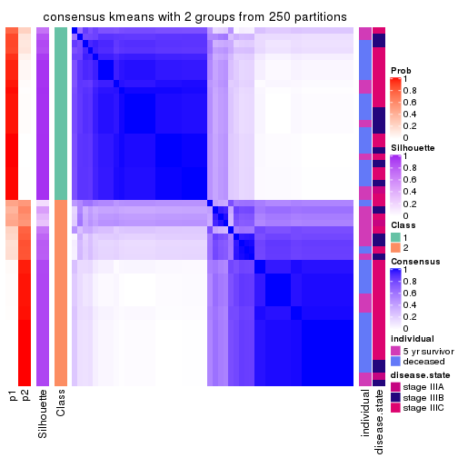
consensus_heatmap(res, k = 3)
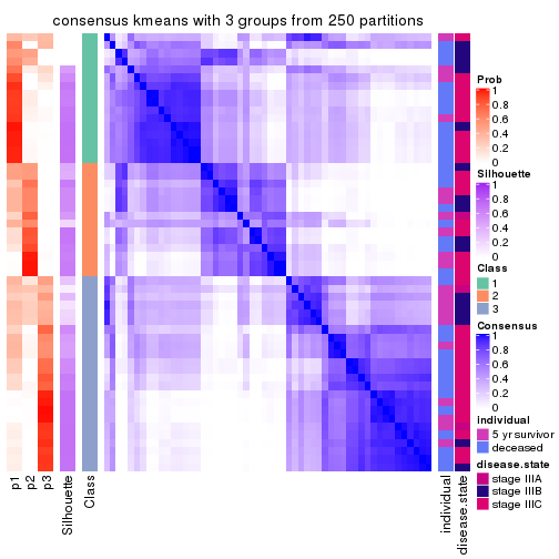
consensus_heatmap(res, k = 4)
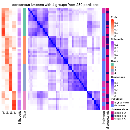
consensus_heatmap(res, k = 5)
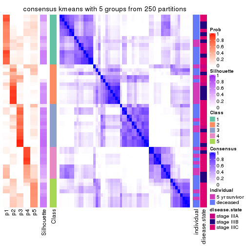
consensus_heatmap(res, k = 6)
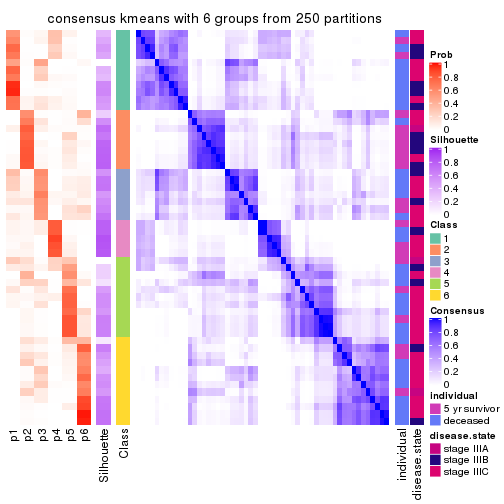
Heatmaps for the membership of samples in all partitions to see how consistent they are:
membership_heatmap(res, k = 2)

membership_heatmap(res, k = 3)
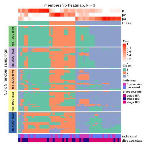
membership_heatmap(res, k = 4)
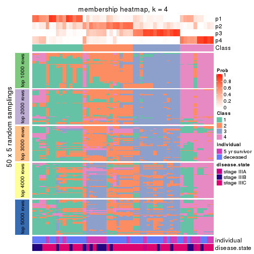
membership_heatmap(res, k = 5)
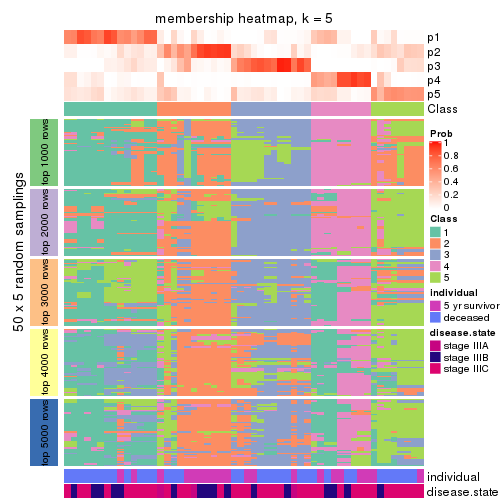
membership_heatmap(res, k = 6)
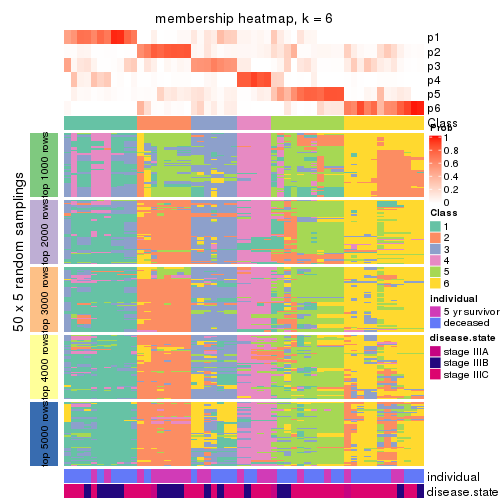
As soon as we have had the classes for columns, we can look for signatures which are significantly different between classes which can be candidate marks for certain classes. Following are the heatmaps for signatures.
Signature heatmaps where rows are scaled:
get_signatures(res, k = 2)
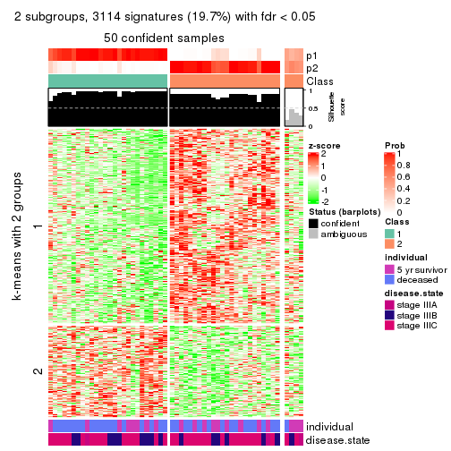
get_signatures(res, k = 3)
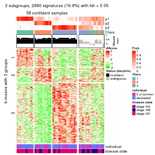
get_signatures(res, k = 4)
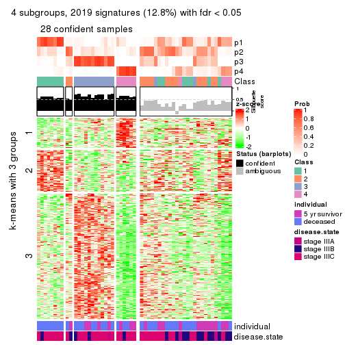
get_signatures(res, k = 5)
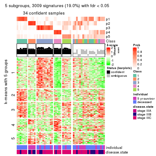
get_signatures(res, k = 6)
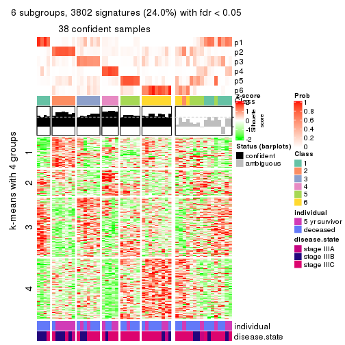
Signature heatmaps where rows are not scaled:
get_signatures(res, k = 2, scale_rows = FALSE)
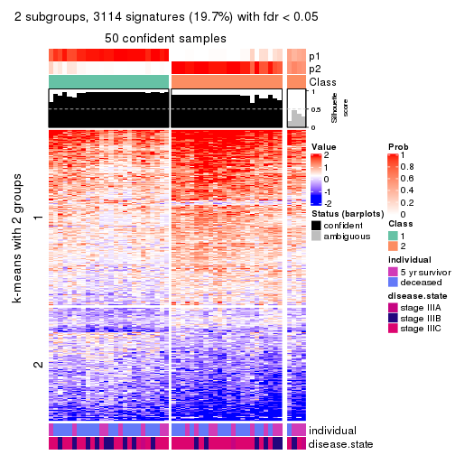
get_signatures(res, k = 3, scale_rows = FALSE)
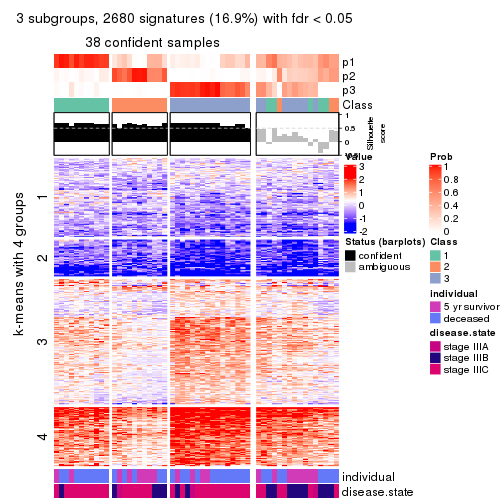
get_signatures(res, k = 4, scale_rows = FALSE)
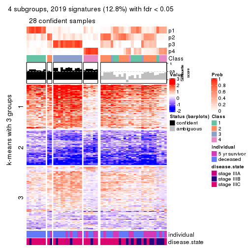
get_signatures(res, k = 5, scale_rows = FALSE)
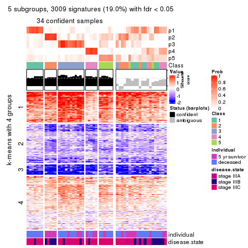
get_signatures(res, k = 6, scale_rows = FALSE)
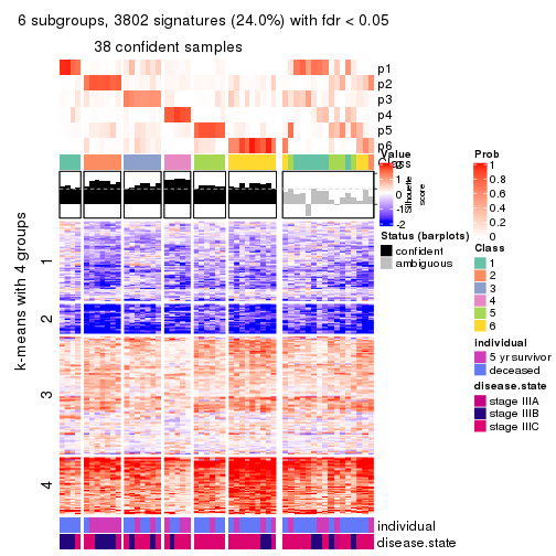
Compare the overlap of signatures from different k:
compare_signatures(res)
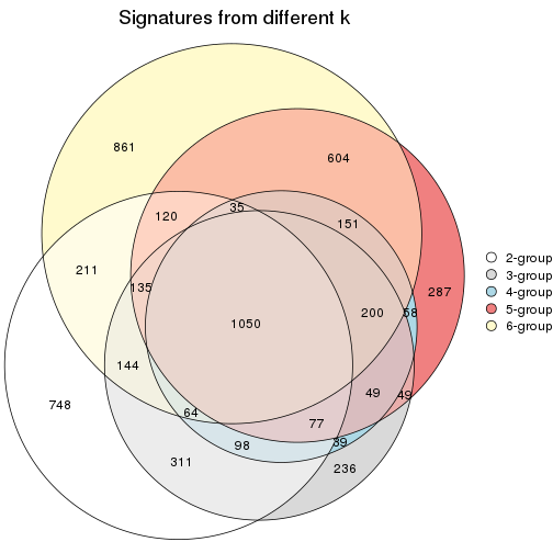
get_signature() returns a data frame invisibly. TO get the list of signatures, the function
call should be assigned to a variable explicitly. In following code, if plot argument is set
to FALSE, no heatmap is plotted while only the differential analysis is performed.
# code only for demonstration
tb = get_signature(res, k = ..., plot = FALSE)
An example of the output of tb is:
#>   which_row         fdr    mean_1    mean_2 scaled_mean_1 scaled_mean_2 km
#> 1        38 0.042760348  8.373488  9.131774    -0.5533452     0.5164555  1
#> 2        40 0.018707592  7.106213  8.469186    -0.6173731     0.5762149  1
#> 3        55 0.019134737 10.221463 11.207825    -0.6159697     0.5749050  1
#> 4        59 0.006059896  5.921854  7.869574    -0.6899429     0.6439467  1
#> 5        60 0.018055526  8.928898 10.211722    -0.6204761     0.5791110  1
#> 6        98 0.009384629 15.714769 14.887706     0.6635654    -0.6193277  2
...
The columns in tb are:
which_row: row indices corresponding to the input matrix.fdr: FDR for the differential test. mean_x: The mean value in group x.scaled_mean_x: The mean value in group x after rows are scaled.km: Row groups if k-means clustering is applied to rows.UMAP plot which shows how samples are separated.
dimension_reduction(res, k = 2, method = "UMAP")
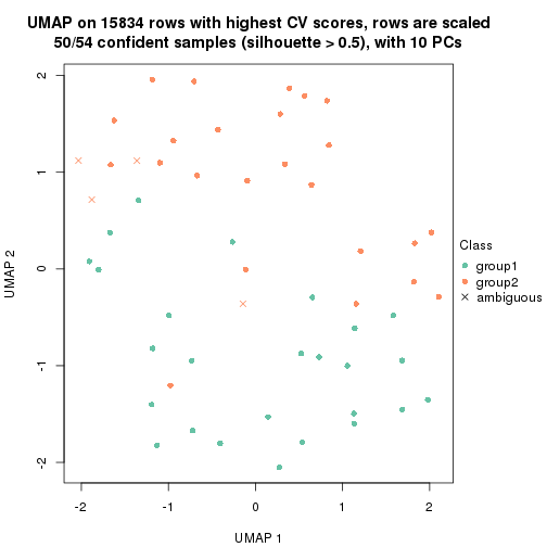
dimension_reduction(res, k = 3, method = "UMAP")
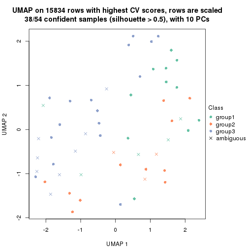
dimension_reduction(res, k = 4, method = "UMAP")
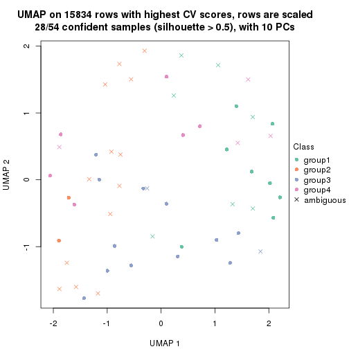
dimension_reduction(res, k = 5, method = "UMAP")
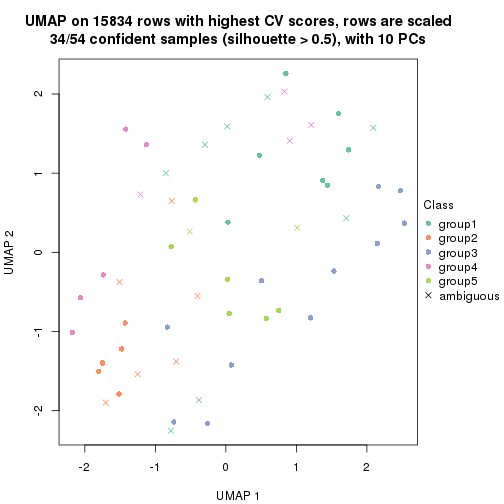
dimension_reduction(res, k = 6, method = "UMAP")
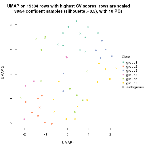
Following heatmap shows how subgroups are split when increasing k:
collect_classes(res)
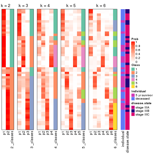
Test correlation between subgroups and known annotations. If the known annotation is numeric, one-way ANOVA test is applied, and if the known annotation is discrete, chi-squared contingency table test is applied.
test_to_known_factors(res)
#>            n individual(p) disease.state(p) k
#> CV:kmeans 50        0.8390           0.7591 2
#> CV:kmeans 38        0.1409           0.3192 3
#> CV:kmeans 28        0.1623           0.8140 4
#> CV:kmeans 34        0.0037           0.0993 5
#> CV:kmeans 38        0.0415           0.2297 6
If matrix rows can be associated to genes, consider to use functional_enrichment(res,
...) to perform function enrichment for the signature genes. See this vignette for more detailed explanations.
The object with results only for a single top-value method and a single partition method can be extracted as:
res = res_list["CV", "skmeans"]
# you can also extract it by
# res = res_list["CV:skmeans"]
A summary of res and all the functions that can be applied to it:
res
#> A 'ConsensusPartition' object with k = 2, 3, 4, 5, 6.
#>   On a matrix with 15834 rows and 54 columns.
#>   Top rows (1000, 2000, 3000, 4000, 5000) are extracted by 'CV' method.
#>   Subgroups are detected by 'skmeans' method.
#>   Performed in total 1250 partitions by row resampling.
#>   Best k for subgroups seems to be 2.
#>
#> Following methods can be applied to this 'ConsensusPartition' object:
#>  [1] "cola_report"             "collect_classes"         "collect_plots"
#>  [4] "collect_stats"           "colnames"                "compare_signatures"
#>  [7] "consensus_heatmap"       "dimension_reduction"     "functional_enrichment"
#> [10] "get_anno_col"            "get_anno"                "get_classes"
#> [13] "get_consensus"           "get_matrix"              "get_membership"
#> [16] "get_param"               "get_signatures"          "get_stats"
#> [19] "is_best_k"               "is_stable_k"             "membership_heatmap"
#> [22] "ncol"                    "nrow"                    "plot_ecdf"
#> [25] "rownames"                "select_partition_number" "show"
#> [28] "suggest_best_k"          "test_to_known_factors"
collect_plots() function collects all the plots made from res for all k (number of partitions)
into one single page to provide an easy and fast comparison between different k.
collect_plots(res)
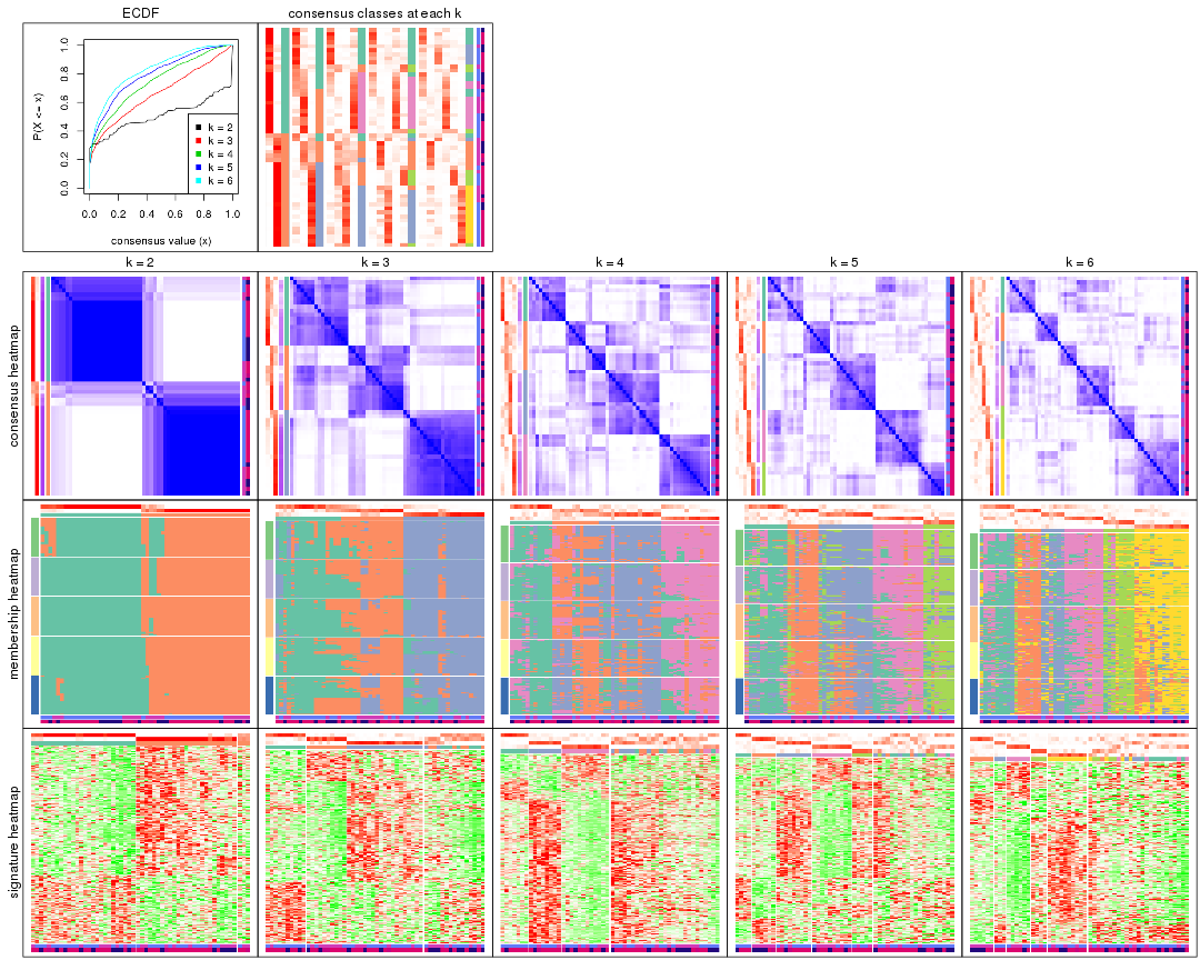
The plots are:
k and the heatmap of
predicted classes for each k.k.k.k.All the plots in panels can be made by individual functions and they are plotted later in this section.
select_partition_number() produces several plots showing different
statistics for choosing “optimized” k. There are following statistics:
k;k, the area increased is defined as \(A_k - A_{k-1}\).The detailed explanations of these statistics can be found in the cola vignette.
Generally speaking, lower PAC score, higher mean silhouette score or higher
concordance corresponds to better partition. Rand index and Jaccard index
measure how similar the current partition is compared to partition with k-1.
If they are too similar, we won't accept k is better than k-1.
select_partition_number(res)
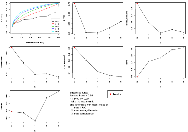
The numeric values for all these statistics can be obtained by get_stats().
get_stats(res)
#>   k 1-PAC mean_silhouette concordance area_increased  Rand Jaccard
#> 2 2 0.752           0.878       0.948         0.5095 0.491   0.491
#> 3 3 0.461           0.591       0.804         0.3089 0.716   0.484
#> 4 4 0.457           0.435       0.697         0.1236 0.772   0.427
#> 5 5 0.507           0.483       0.703         0.0664 0.887   0.589
#> 6 6 0.571           0.444       0.673         0.0404 0.919   0.633
suggest_best_k() suggests the best \(k\) based on these statistics. The rules are as follows:
suggest_best_k(res)
#> [1] 2
Following shows the table of the partitions (You need to click the show/hide
code output link to see it). The membership matrix (columns with name p*)
is inferred by
clue::cl_consensus()
function with the SE method. Basically the value in the membership matrix
represents the probability to belong to a certain group. The finall class
label for an item is determined with the group with highest probability it
belongs to.
In get_classes() function, the entropy is calculated from the membership
matrix and the silhouette score is calculated from the consensus matrix.
cbind(get_classes(res, k = 2), get_membership(res, k = 2))
#>           class entropy silhouette    p1    p2
#> GSM311939     2  0.0000      0.921 0.000 1.000
#> GSM311963     2  0.9993      0.145 0.484 0.516
#> GSM311973     1  0.0000      0.964 1.000 0.000
#> GSM311940     2  0.0000      0.921 0.000 1.000
#> GSM311953     2  0.6887      0.757 0.184 0.816
#> GSM311974     2  0.0000      0.921 0.000 1.000
#> GSM311975     1  0.4431      0.881 0.908 0.092
#> GSM311977     2  0.7528      0.720 0.216 0.784
#> GSM311982     1  0.0000      0.964 1.000 0.000
#> GSM311990     2  0.0000      0.921 0.000 1.000
#> GSM311943     2  0.8081      0.649 0.248 0.752
#> GSM311944     1  0.7219      0.755 0.800 0.200
#> GSM311946     2  0.9732      0.381 0.404 0.596
#> GSM311956     1  0.3584      0.907 0.932 0.068
#> GSM311967     2  0.0000      0.921 0.000 1.000
#> GSM311968     2  0.0000      0.921 0.000 1.000
#> GSM311972     1  0.0000      0.964 1.000 0.000
#> GSM311980     1  0.0000      0.964 1.000 0.000
#> GSM311981     1  0.0000      0.964 1.000 0.000
#> GSM311988     2  0.0000      0.921 0.000 1.000
#> GSM311957     2  0.0938      0.913 0.012 0.988
#> GSM311960     1  0.0000      0.964 1.000 0.000
#> GSM311971     1  0.0000      0.964 1.000 0.000
#> GSM311976     1  0.0000      0.964 1.000 0.000
#> GSM311978     1  0.0000      0.964 1.000 0.000
#> GSM311979     1  0.0000      0.964 1.000 0.000
#> GSM311983     1  0.6531      0.801 0.832 0.168
#> GSM311986     2  0.0000      0.921 0.000 1.000
#> GSM311991     1  0.0000      0.964 1.000 0.000
#> GSM311938     2  0.0000      0.921 0.000 1.000
#> GSM311941     2  0.0000      0.921 0.000 1.000
#> GSM311942     2  0.0000      0.921 0.000 1.000
#> GSM311945     1  0.0000      0.964 1.000 0.000
#> GSM311947     2  0.0000      0.921 0.000 1.000
#> GSM311948     2  0.0000      0.921 0.000 1.000
#> GSM311949     1  0.0000      0.964 1.000 0.000
#> GSM311950     2  0.0000      0.921 0.000 1.000
#> GSM311951     2  0.0000      0.921 0.000 1.000
#> GSM311952     1  0.0000      0.964 1.000 0.000
#> GSM311954     2  0.0000      0.921 0.000 1.000
#> GSM311955     1  0.5629      0.848 0.868 0.132
#> GSM311958     1  0.0000      0.964 1.000 0.000
#> GSM311959     2  0.0376      0.919 0.004 0.996
#> GSM311961     2  0.9963      0.163 0.464 0.536
#> GSM311962     1  0.0000      0.964 1.000 0.000
#> GSM311964     1  0.0000      0.964 1.000 0.000
#> GSM311965     2  0.0000      0.921 0.000 1.000
#> GSM311966     1  0.0000      0.964 1.000 0.000
#> GSM311969     2  0.0000      0.921 0.000 1.000
#> GSM311970     1  0.0000      0.964 1.000 0.000
#> GSM311984     2  0.0000      0.921 0.000 1.000
#> GSM311985     1  0.0000      0.964 1.000 0.000
#> GSM311987     2  0.0000      0.921 0.000 1.000
#> GSM311989     1  0.5737      0.843 0.864 0.136
cbind(get_classes(res, k = 3), get_membership(res, k = 3))
#>           class entropy silhouette    p1    p2    p3
#> GSM311939     3  0.0661     0.8581 0.008 0.004 0.988
#> GSM311963     2  0.6565     0.5657 0.048 0.720 0.232
#> GSM311973     2  0.1529     0.6541 0.040 0.960 0.000
#> GSM311940     3  0.6520    -0.0429 0.004 0.488 0.508
#> GSM311953     2  0.6738     0.3773 0.020 0.624 0.356
#> GSM311974     2  0.6264     0.3252 0.004 0.616 0.380
#> GSM311975     1  0.8520     0.2916 0.588 0.280 0.132
#> GSM311977     2  0.5690     0.5417 0.004 0.708 0.288
#> GSM311982     1  0.6308     0.2432 0.508 0.492 0.000
#> GSM311990     3  0.0892     0.8610 0.020 0.000 0.980
#> GSM311943     1  0.6154     0.0632 0.592 0.000 0.408
#> GSM311944     1  0.6827     0.5975 0.728 0.080 0.192
#> GSM311946     2  0.4974     0.5683 0.000 0.764 0.236
#> GSM311956     2  0.1482     0.6518 0.012 0.968 0.020
#> GSM311967     3  0.0592     0.8556 0.000 0.012 0.988
#> GSM311968     3  0.5339     0.8185 0.096 0.080 0.824
#> GSM311972     1  0.6274     0.3088 0.544 0.456 0.000
#> GSM311980     2  0.1529     0.6549 0.040 0.960 0.000
#> GSM311981     2  0.4555     0.5109 0.200 0.800 0.000
#> GSM311988     3  0.1525     0.8517 0.004 0.032 0.964
#> GSM311957     3  0.5331     0.7806 0.184 0.024 0.792
#> GSM311960     2  0.1411     0.6558 0.036 0.964 0.000
#> GSM311971     1  0.5988     0.4353 0.632 0.368 0.000
#> GSM311976     2  0.6274    -0.0295 0.456 0.544 0.000
#> GSM311978     1  0.5291     0.5620 0.732 0.268 0.000
#> GSM311979     1  0.6192     0.3745 0.580 0.420 0.000
#> GSM311983     1  0.1267     0.6676 0.972 0.004 0.024
#> GSM311986     3  0.3038     0.8405 0.104 0.000 0.896
#> GSM311991     2  0.5706     0.3245 0.320 0.680 0.000
#> GSM311938     3  0.1647     0.8470 0.004 0.036 0.960
#> GSM311941     3  0.2878     0.8446 0.096 0.000 0.904
#> GSM311942     3  0.4172     0.8393 0.104 0.028 0.868
#> GSM311945     2  0.2165     0.6433 0.064 0.936 0.000
#> GSM311947     3  0.1267     0.8534 0.004 0.024 0.972
#> GSM311948     3  0.6818     0.3816 0.024 0.348 0.628
#> GSM311949     2  0.6140     0.1354 0.404 0.596 0.000
#> GSM311950     3  0.0747     0.8545 0.000 0.016 0.984
#> GSM311951     3  0.1525     0.8510 0.004 0.032 0.964
#> GSM311952     1  0.1411     0.6744 0.964 0.036 0.000
#> GSM311954     3  0.2772     0.8535 0.080 0.004 0.916
#> GSM311955     1  0.3649     0.6505 0.896 0.036 0.068
#> GSM311958     1  0.0892     0.6737 0.980 0.020 0.000
#> GSM311959     3  0.5431     0.6486 0.284 0.000 0.716
#> GSM311961     1  0.7298     0.5308 0.692 0.088 0.220
#> GSM311962     1  0.0475     0.6712 0.992 0.004 0.004
#> GSM311964     2  0.5835     0.2542 0.340 0.660 0.000
#> GSM311965     3  0.3995     0.8096 0.016 0.116 0.868
#> GSM311966     1  0.3116     0.6571 0.892 0.108 0.000
#> GSM311969     3  0.5650     0.6047 0.312 0.000 0.688
#> GSM311970     2  0.1643     0.6543 0.044 0.956 0.000
#> GSM311984     3  0.1267     0.8601 0.024 0.004 0.972
#> GSM311985     1  0.3619     0.6483 0.864 0.136 0.000
#> GSM311987     3  0.2625     0.8502 0.084 0.000 0.916
#> GSM311989     1  0.7768     0.4334 0.592 0.344 0.064
cbind(get_classes(res, k = 4), get_membership(res, k = 4))
#>           class entropy silhouette    p1    p2    p3    p4
#> GSM311939     3  0.2984     0.5837 0.028 0.084 0.888 0.000
#> GSM311963     3  0.8196    -0.2981 0.008 0.328 0.340 0.324
#> GSM311973     4  0.4034     0.6434 0.008 0.192 0.004 0.796
#> GSM311940     2  0.6985     0.1559 0.000 0.480 0.404 0.116
#> GSM311953     2  0.7394     0.2466 0.004 0.508 0.328 0.160
#> GSM311974     2  0.6281     0.3066 0.000 0.656 0.216 0.128
#> GSM311975     1  0.8321     0.2770 0.484 0.076 0.108 0.332
#> GSM311977     2  0.7894     0.2175 0.000 0.376 0.320 0.304
#> GSM311982     4  0.5130     0.5194 0.332 0.016 0.000 0.652
#> GSM311990     3  0.4155     0.4943 0.004 0.240 0.756 0.000
#> GSM311943     1  0.6123     0.2026 0.600 0.064 0.336 0.000
#> GSM311944     2  0.8290    -0.1222 0.404 0.420 0.116 0.060
#> GSM311946     2  0.7803     0.2532 0.000 0.416 0.268 0.316
#> GSM311956     4  0.3048     0.6731 0.000 0.108 0.016 0.876
#> GSM311967     3  0.3004     0.5850 0.008 0.100 0.884 0.008
#> GSM311968     2  0.5511     0.1245 0.008 0.604 0.376 0.012
#> GSM311972     4  0.3907     0.6403 0.232 0.000 0.000 0.768
#> GSM311980     4  0.2164     0.6999 0.004 0.068 0.004 0.924
#> GSM311981     4  0.1743     0.7164 0.056 0.004 0.000 0.940
#> GSM311988     3  0.3942     0.4310 0.000 0.236 0.764 0.000
#> GSM311957     3  0.7459     0.3709 0.192 0.280 0.524 0.004
#> GSM311960     4  0.3764     0.6376 0.000 0.216 0.000 0.784
#> GSM311971     4  0.5408     0.2327 0.488 0.012 0.000 0.500
#> GSM311976     4  0.4718     0.6089 0.280 0.012 0.000 0.708
#> GSM311978     1  0.5132    -0.1196 0.548 0.004 0.000 0.448
#> GSM311979     4  0.5004     0.4317 0.392 0.004 0.000 0.604
#> GSM311983     1  0.1520     0.6990 0.956 0.000 0.024 0.020
#> GSM311986     3  0.4374     0.6100 0.120 0.068 0.812 0.000
#> GSM311991     4  0.2530     0.7142 0.100 0.004 0.000 0.896
#> GSM311938     3  0.4612     0.4243 0.016 0.212 0.764 0.008
#> GSM311941     3  0.5184     0.5372 0.060 0.204 0.736 0.000
#> GSM311942     2  0.5050     0.0819 0.004 0.588 0.408 0.000
#> GSM311945     4  0.5767     0.3221 0.016 0.436 0.008 0.540
#> GSM311947     3  0.5284     0.1095 0.004 0.436 0.556 0.004
#> GSM311948     2  0.4375     0.3157 0.008 0.812 0.144 0.036
#> GSM311949     4  0.4644     0.6592 0.208 0.024 0.004 0.764
#> GSM311950     3  0.1978     0.5832 0.000 0.068 0.928 0.004
#> GSM311951     2  0.4855     0.0851 0.000 0.600 0.400 0.000
#> GSM311952     1  0.3606     0.6500 0.844 0.024 0.000 0.132
#> GSM311954     3  0.3080     0.6279 0.096 0.024 0.880 0.000
#> GSM311955     1  0.4017     0.6769 0.860 0.036 0.052 0.052
#> GSM311958     1  0.1743     0.6958 0.940 0.004 0.000 0.056
#> GSM311959     3  0.6002     0.4947 0.268 0.068 0.660 0.004
#> GSM311961     1  0.7985     0.4712 0.580 0.084 0.220 0.116
#> GSM311962     1  0.0817     0.6975 0.976 0.000 0.000 0.024
#> GSM311964     4  0.2647     0.7096 0.120 0.000 0.000 0.880
#> GSM311965     2  0.5696     0.1194 0.004 0.592 0.380 0.024
#> GSM311966     1  0.2999     0.6351 0.864 0.004 0.000 0.132
#> GSM311969     3  0.6162     0.4620 0.304 0.076 0.620 0.000
#> GSM311970     4  0.1297     0.7035 0.000 0.020 0.016 0.964
#> GSM311984     3  0.3716     0.6180 0.096 0.052 0.852 0.000
#> GSM311985     1  0.4123     0.5640 0.772 0.008 0.000 0.220
#> GSM311987     3  0.3612     0.6234 0.100 0.044 0.856 0.000
#> GSM311989     2  0.8354     0.0620 0.224 0.500 0.044 0.232
cbind(get_classes(res, k = 5), get_membership(res, k = 5))
#>           class entropy silhouette    p1    p2    p3    p4    p5
#> GSM311939     3   0.391     0.5756 0.000 0.272 0.720 0.000 0.008
#> GSM311963     2   0.469     0.6547 0.052 0.772 0.028 0.144 0.004
#> GSM311973     4   0.606     0.5422 0.052 0.172 0.004 0.672 0.100
#> GSM311940     2   0.287     0.6752 0.000 0.884 0.060 0.008 0.048
#> GSM311953     2   0.159     0.7180 0.000 0.948 0.008 0.028 0.016
#> GSM311974     2   0.427     0.6321 0.000 0.776 0.004 0.068 0.152
#> GSM311975     1   0.940     0.1978 0.312 0.192 0.080 0.276 0.140
#> GSM311977     2   0.234     0.7175 0.004 0.904 0.008 0.080 0.004
#> GSM311982     4   0.503     0.5123 0.292 0.016 0.000 0.660 0.032
#> GSM311990     3   0.507     0.4498 0.000 0.064 0.648 0.000 0.288
#> GSM311943     3   0.710     0.0571 0.300 0.036 0.500 0.004 0.160
#> GSM311944     5   0.519     0.5397 0.180 0.004 0.052 0.036 0.728
#> GSM311946     2   0.289     0.7090 0.000 0.864 0.004 0.116 0.016
#> GSM311956     4   0.332     0.6256 0.000 0.160 0.000 0.820 0.020
#> GSM311967     3   0.611     0.5500 0.000 0.216 0.608 0.012 0.164
#> GSM311968     5   0.419     0.6905 0.004 0.020 0.148 0.032 0.796
#> GSM311972     4   0.403     0.5816 0.236 0.000 0.004 0.744 0.016
#> GSM311980     4   0.287     0.6570 0.004 0.100 0.000 0.872 0.024
#> GSM311981     4   0.316     0.6687 0.048 0.048 0.008 0.880 0.016
#> GSM311988     2   0.516    -0.2245 0.000 0.512 0.448 0.000 0.040
#> GSM311957     3   0.838     0.2116 0.168 0.140 0.448 0.020 0.224
#> GSM311960     4   0.594     0.5491 0.028 0.112 0.004 0.664 0.192
#> GSM311971     1   0.571     0.0622 0.584 0.012 0.008 0.348 0.048
#> GSM311976     4   0.561     0.2903 0.424 0.020 0.004 0.524 0.028
#> GSM311978     1   0.494     0.1424 0.624 0.004 0.004 0.344 0.024
#> GSM311979     4   0.500     0.3150 0.424 0.004 0.000 0.548 0.024
#> GSM311983     1   0.346     0.5763 0.856 0.016 0.092 0.008 0.028
#> GSM311986     3   0.236     0.6665 0.024 0.032 0.916 0.000 0.028
#> GSM311991     4   0.300     0.6654 0.088 0.020 0.004 0.876 0.012
#> GSM311938     3   0.506     0.2054 0.012 0.480 0.496 0.004 0.008
#> GSM311941     3   0.402     0.5836 0.000 0.036 0.764 0.000 0.200
#> GSM311942     5   0.316     0.6702 0.000 0.004 0.188 0.000 0.808
#> GSM311945     5   0.546    -0.0324 0.004 0.040 0.004 0.448 0.504
#> GSM311947     5   0.601     0.2918 0.000 0.120 0.320 0.004 0.556
#> GSM311948     2   0.571     0.0398 0.000 0.492 0.032 0.028 0.448
#> GSM311949     4   0.553     0.4379 0.324 0.020 0.008 0.616 0.032
#> GSM311950     3   0.584     0.4984 0.000 0.316 0.576 0.004 0.104
#> GSM311951     5   0.337     0.6772 0.000 0.008 0.180 0.004 0.808
#> GSM311952     1   0.766     0.4698 0.572 0.048 0.128 0.172 0.080
#> GSM311954     3   0.265     0.6706 0.004 0.124 0.868 0.004 0.000
#> GSM311955     1   0.824     0.3292 0.440 0.052 0.296 0.056 0.156
#> GSM311958     1   0.625     0.5464 0.696 0.028 0.116 0.080 0.080
#> GSM311959     3   0.259     0.6255 0.064 0.000 0.896 0.004 0.036
#> GSM311961     1   0.880     0.2428 0.396 0.120 0.300 0.112 0.072
#> GSM311962     1   0.230     0.5664 0.916 0.004 0.048 0.028 0.004
#> GSM311964     4   0.365     0.6516 0.164 0.016 0.000 0.808 0.012
#> GSM311965     5   0.407     0.6900 0.004 0.028 0.144 0.020 0.804
#> GSM311966     1   0.311     0.5122 0.864 0.004 0.008 0.104 0.020
#> GSM311969     3   0.314     0.5974 0.108 0.000 0.852 0.000 0.040
#> GSM311970     4   0.211     0.6662 0.004 0.084 0.000 0.908 0.004
#> GSM311984     3   0.490     0.6188 0.040 0.184 0.744 0.008 0.024
#> GSM311985     1   0.514     0.4124 0.696 0.000 0.008 0.212 0.084
#> GSM311987     3   0.214     0.6772 0.004 0.064 0.916 0.000 0.016
#> GSM311989     5   0.650     0.4347 0.148 0.024 0.036 0.140 0.652
cbind(get_classes(res, k = 6), get_membership(res, k = 6))
#>           class entropy silhouette    p1    p2    p3    p4    p5    p6
#> GSM311939     6   0.387    0.61041 0.008 0.220 0.016 0.000 0.008 0.748
#> GSM311963     2   0.641    0.59194 0.052 0.624 0.068 0.192 0.008 0.056
#> GSM311973     4   0.619    0.48754 0.116 0.116 0.036 0.648 0.084 0.000
#> GSM311940     2   0.469    0.61381 0.012 0.768 0.032 0.020 0.044 0.124
#> GSM311953     2   0.225    0.71361 0.004 0.916 0.004 0.024 0.024 0.028
#> GSM311974     2   0.443    0.63464 0.000 0.744 0.016 0.072 0.164 0.004
#> GSM311975     3   0.911    0.09844 0.172 0.112 0.340 0.232 0.076 0.068
#> GSM311977     2   0.486    0.70137 0.040 0.772 0.032 0.092 0.016 0.048
#> GSM311982     4   0.513    0.22806 0.384 0.008 0.036 0.556 0.016 0.000
#> GSM311990     6   0.404    0.56275 0.004 0.040 0.000 0.000 0.232 0.724
#> GSM311943     3   0.484    0.45951 0.036 0.000 0.660 0.000 0.036 0.268
#> GSM311944     5   0.524    0.49649 0.224 0.004 0.068 0.016 0.672 0.016
#> GSM311946     2   0.381    0.69102 0.004 0.792 0.024 0.152 0.028 0.000
#> GSM311956     4   0.362    0.59891 0.004 0.148 0.024 0.804 0.020 0.000
#> GSM311967     6   0.629    0.55576 0.020 0.168 0.052 0.004 0.140 0.616
#> GSM311968     5   0.385    0.63060 0.008 0.036 0.016 0.040 0.832 0.068
#> GSM311972     4   0.480    0.35719 0.308 0.004 0.048 0.632 0.008 0.000
#> GSM311980     4   0.257    0.63864 0.000 0.064 0.020 0.888 0.028 0.000
#> GSM311981     4   0.385    0.61103 0.104 0.012 0.064 0.808 0.012 0.000
#> GSM311988     6   0.527    0.36775 0.000 0.400 0.028 0.004 0.036 0.532
#> GSM311957     6   0.868    0.17790 0.128 0.124 0.156 0.012 0.200 0.380
#> GSM311960     4   0.674    0.45693 0.060 0.120 0.064 0.604 0.148 0.004
#> GSM311971     1   0.416    0.44698 0.744 0.004 0.028 0.204 0.020 0.000
#> GSM311976     1   0.647    0.13957 0.456 0.028 0.112 0.384 0.016 0.004
#> GSM311978     1   0.398    0.45499 0.744 0.004 0.036 0.212 0.004 0.000
#> GSM311979     1   0.464    0.03907 0.524 0.004 0.032 0.440 0.000 0.000
#> GSM311983     3   0.520    0.31826 0.420 0.008 0.520 0.004 0.008 0.040
#> GSM311986     6   0.285    0.67304 0.000 0.020 0.064 0.000 0.044 0.872
#> GSM311991     4   0.383    0.58641 0.136 0.004 0.060 0.792 0.008 0.000
#> GSM311938     6   0.547    0.32159 0.016 0.400 0.052 0.000 0.012 0.520
#> GSM311941     6   0.403    0.56401 0.000 0.016 0.016 0.004 0.232 0.732
#> GSM311942     5   0.310    0.63111 0.004 0.016 0.008 0.000 0.832 0.140
#> GSM311945     5   0.702   -0.07110 0.048 0.052 0.072 0.404 0.416 0.008
#> GSM311947     5   0.614    0.26364 0.008 0.120 0.032 0.000 0.536 0.304
#> GSM311948     2   0.660    0.04211 0.040 0.444 0.024 0.036 0.420 0.036
#> GSM311949     1   0.609    0.00782 0.452 0.052 0.044 0.432 0.020 0.000
#> GSM311950     6   0.552    0.56980 0.008 0.228 0.020 0.000 0.112 0.632
#> GSM311951     5   0.336    0.64204 0.012 0.036 0.012 0.004 0.848 0.088
#> GSM311952     3   0.510    0.56346 0.168 0.004 0.716 0.064 0.016 0.032
#> GSM311954     6   0.213    0.68054 0.004 0.052 0.028 0.000 0.004 0.912
#> GSM311955     3   0.576    0.58162 0.116 0.012 0.692 0.028 0.040 0.112
#> GSM311958     3   0.506    0.52561 0.244 0.004 0.672 0.048 0.008 0.024
#> GSM311959     6   0.386    0.54348 0.004 0.004 0.216 0.000 0.028 0.748
#> GSM311961     1   0.881   -0.20573 0.320 0.100 0.252 0.044 0.056 0.228
#> GSM311962     1   0.440   -0.20031 0.576 0.000 0.400 0.000 0.008 0.016
#> GSM311964     4   0.346    0.51959 0.240 0.004 0.008 0.748 0.000 0.000
#> GSM311965     5   0.423    0.64051 0.048 0.028 0.012 0.020 0.808 0.084
#> GSM311966     1   0.326    0.32276 0.820 0.000 0.144 0.024 0.012 0.000
#> GSM311969     6   0.451    0.43158 0.016 0.008 0.284 0.000 0.020 0.672
#> GSM311970     4   0.209    0.65035 0.020 0.036 0.020 0.920 0.004 0.000
#> GSM311984     6   0.502    0.62619 0.056 0.080 0.084 0.000 0.032 0.748
#> GSM311985     1   0.559    0.35622 0.688 0.004 0.108 0.120 0.072 0.008
#> GSM311987     6   0.168    0.67626 0.000 0.008 0.032 0.000 0.024 0.936
#> GSM311989     5   0.717    0.33448 0.096 0.016 0.216 0.148 0.516 0.008
Heatmaps for the consensus matrix. It visualizes the probability of two samples to be in a same group.
consensus_heatmap(res, k = 2)
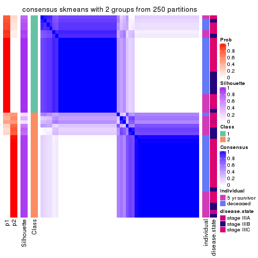
consensus_heatmap(res, k = 3)
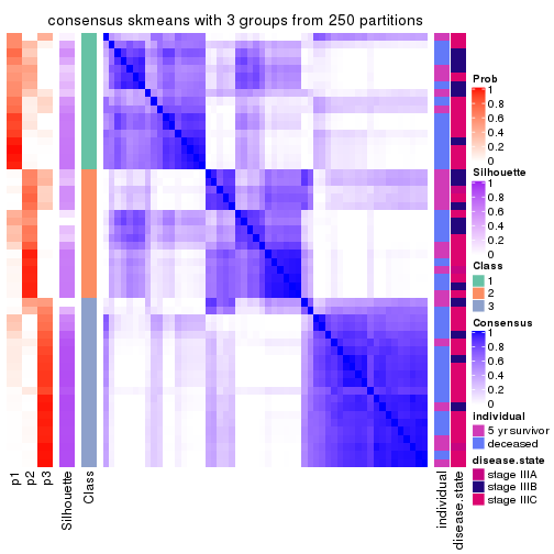
consensus_heatmap(res, k = 4)
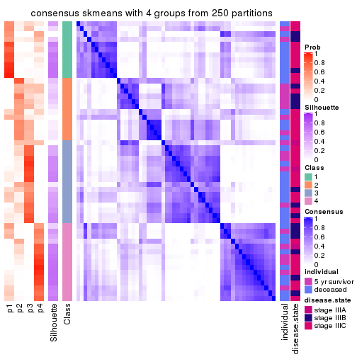
consensus_heatmap(res, k = 5)
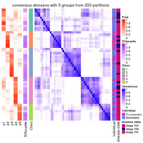
consensus_heatmap(res, k = 6)
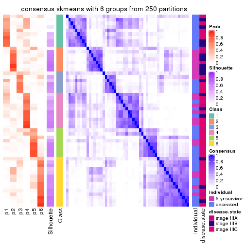
Heatmaps for the membership of samples in all partitions to see how consistent they are:
membership_heatmap(res, k = 2)
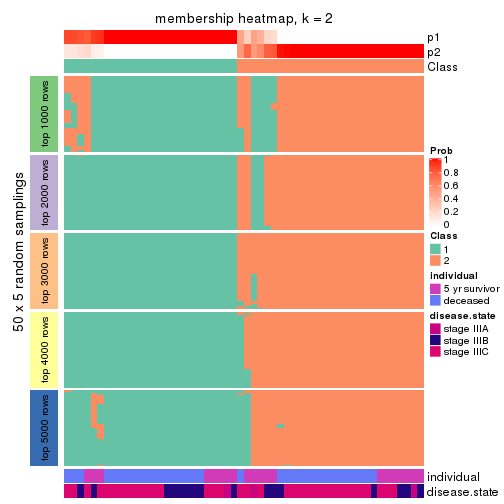
membership_heatmap(res, k = 3)
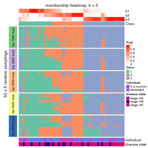
membership_heatmap(res, k = 4)
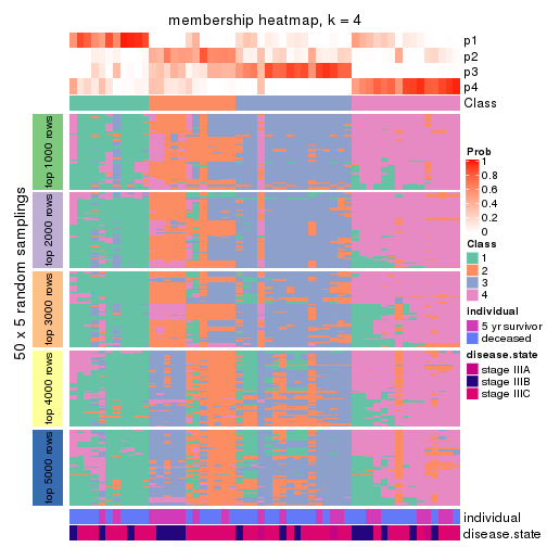
membership_heatmap(res, k = 5)
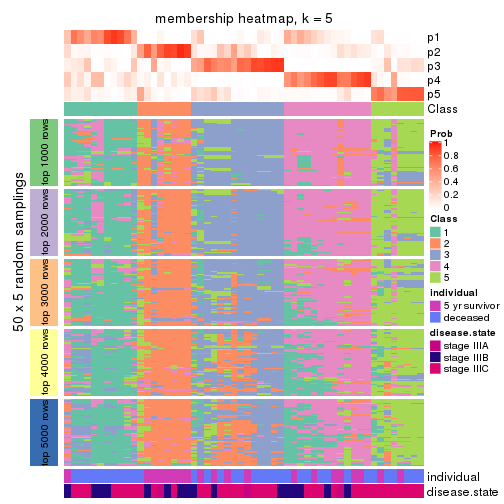
membership_heatmap(res, k = 6)
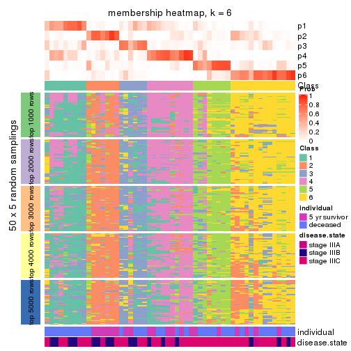
As soon as we have had the classes for columns, we can look for signatures which are significantly different between classes which can be candidate marks for certain classes. Following are the heatmaps for signatures.
Signature heatmaps where rows are scaled:
get_signatures(res, k = 2)
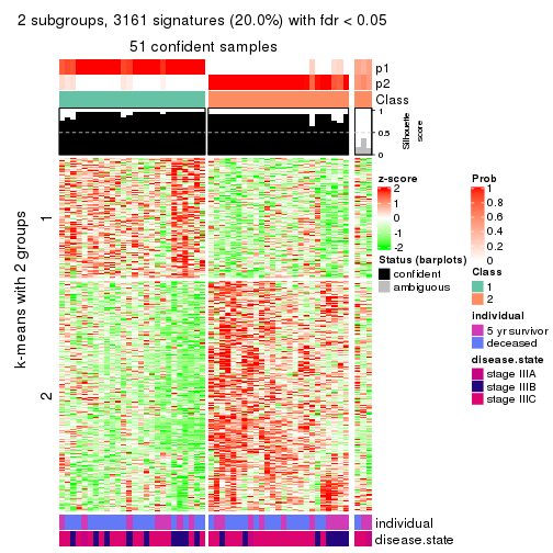
get_signatures(res, k = 3)
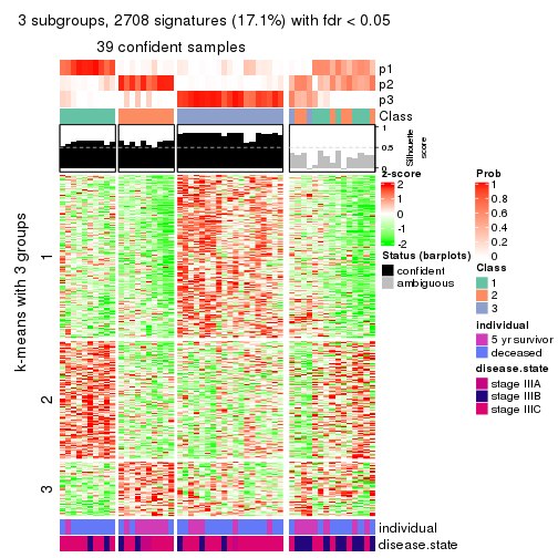
get_signatures(res, k = 4)
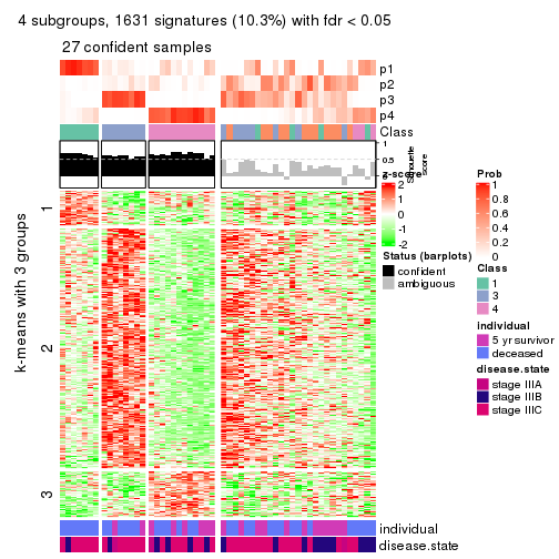
get_signatures(res, k = 5)
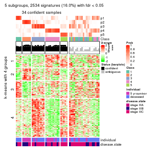
get_signatures(res, k = 6)
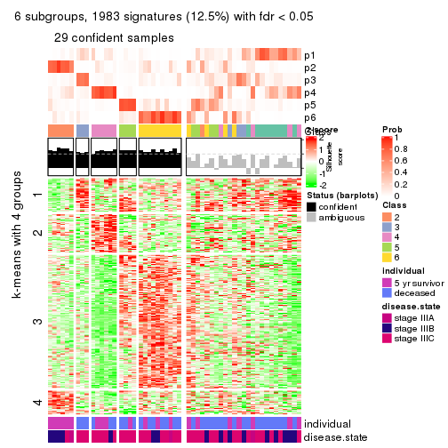
Signature heatmaps where rows are not scaled:
get_signatures(res, k = 2, scale_rows = FALSE)
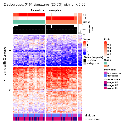
get_signatures(res, k = 3, scale_rows = FALSE)
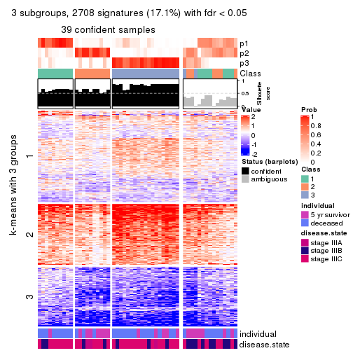
get_signatures(res, k = 4, scale_rows = FALSE)
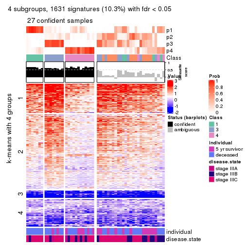
get_signatures(res, k = 5, scale_rows = FALSE)
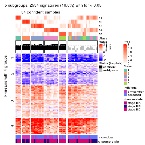
get_signatures(res, k = 6, scale_rows = FALSE)
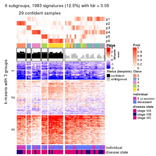
Compare the overlap of signatures from different k:
compare_signatures(res)
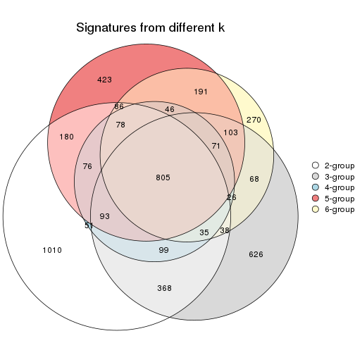
get_signature() returns a data frame invisibly. TO get the list of signatures, the function
call should be assigned to a variable explicitly. In following code, if plot argument is set
to FALSE, no heatmap is plotted while only the differential analysis is performed.
# code only for demonstration
tb = get_signature(res, k = ..., plot = FALSE)
An example of the output of tb is:
#>   which_row         fdr    mean_1    mean_2 scaled_mean_1 scaled_mean_2 km
#> 1        38 0.042760348  8.373488  9.131774    -0.5533452     0.5164555  1
#> 2        40 0.018707592  7.106213  8.469186    -0.6173731     0.5762149  1
#> 3        55 0.019134737 10.221463 11.207825    -0.6159697     0.5749050  1
#> 4        59 0.006059896  5.921854  7.869574    -0.6899429     0.6439467  1
#> 5        60 0.018055526  8.928898 10.211722    -0.6204761     0.5791110  1
#> 6        98 0.009384629 15.714769 14.887706     0.6635654    -0.6193277  2
...
The columns in tb are:
which_row: row indices corresponding to the input matrix.fdr: FDR for the differential test. mean_x: The mean value in group x.scaled_mean_x: The mean value in group x after rows are scaled.km: Row groups if k-means clustering is applied to rows.UMAP plot which shows how samples are separated.
dimension_reduction(res, k = 2, method = "UMAP")
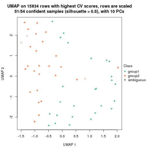
dimension_reduction(res, k = 3, method = "UMAP")
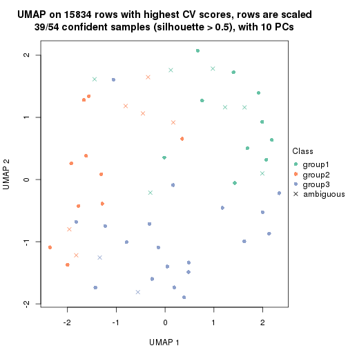
dimension_reduction(res, k = 4, method = "UMAP")
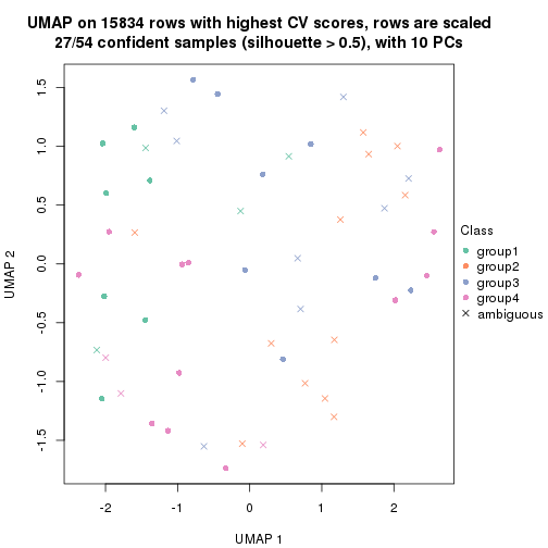
dimension_reduction(res, k = 5, method = "UMAP")
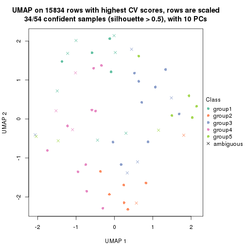
dimension_reduction(res, k = 6, method = "UMAP")
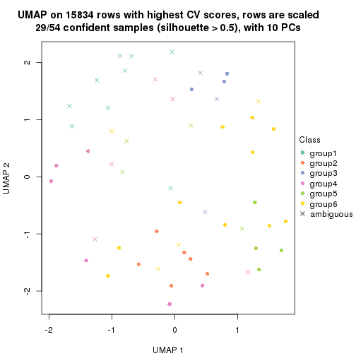
Following heatmap shows how subgroups are split when increasing k:
collect_classes(res)
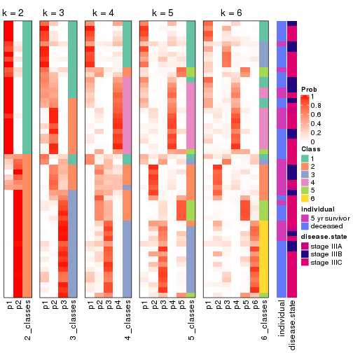
Test correlation between subgroups and known annotations. If the known annotation is numeric, one-way ANOVA test is applied, and if the known annotation is discrete, chi-squared contingency table test is applied.
test_to_known_factors(res)
#>             n individual(p) disease.state(p) k
#> CV:skmeans 51       0.69173            0.878 2
#> CV:skmeans 39       0.01156            0.500 3
#> CV:skmeans 27       0.06661            0.640 4
#> CV:skmeans 34       0.00987            0.228 5
#> CV:skmeans 29       0.02231            0.160 6
If matrix rows can be associated to genes, consider to use functional_enrichment(res,
...) to perform function enrichment for the signature genes. See this vignette for more detailed explanations.
The object with results only for a single top-value method and a single partition method can be extracted as:
res = res_list["CV", "pam"]
# you can also extract it by
# res = res_list["CV:pam"]
A summary of res and all the functions that can be applied to it:
res
#> A 'ConsensusPartition' object with k = 2, 3, 4, 5, 6.
#>   On a matrix with 15834 rows and 54 columns.
#>   Top rows (1000, 2000, 3000, 4000, 5000) are extracted by 'CV' method.
#>   Subgroups are detected by 'pam' method.
#>   Performed in total 1250 partitions by row resampling.
#>   Best k for subgroups seems to be 2.
#>
#> Following methods can be applied to this 'ConsensusPartition' object:
#>  [1] "cola_report"             "collect_classes"         "collect_plots"
#>  [4] "collect_stats"           "colnames"                "compare_signatures"
#>  [7] "consensus_heatmap"       "dimension_reduction"     "functional_enrichment"
#> [10] "get_anno_col"            "get_anno"                "get_classes"
#> [13] "get_consensus"           "get_matrix"              "get_membership"
#> [16] "get_param"               "get_signatures"          "get_stats"
#> [19] "is_best_k"               "is_stable_k"             "membership_heatmap"
#> [22] "ncol"                    "nrow"                    "plot_ecdf"
#> [25] "rownames"                "select_partition_number" "show"
#> [28] "suggest_best_k"          "test_to_known_factors"
collect_plots() function collects all the plots made from res for all k (number of partitions)
into one single page to provide an easy and fast comparison between different k.
collect_plots(res)
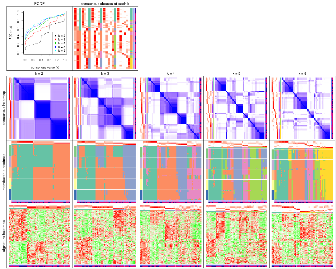
The plots are:
k and the heatmap of
predicted classes for each k.k.k.k.All the plots in panels can be made by individual functions and they are plotted later in this section.
select_partition_number() produces several plots showing different
statistics for choosing “optimized” k. There are following statistics:
k;k, the area increased is defined as \(A_k - A_{k-1}\).The detailed explanations of these statistics can be found in the cola vignette.
Generally speaking, lower PAC score, higher mean silhouette score or higher
concordance corresponds to better partition. Rand index and Jaccard index
measure how similar the current partition is compared to partition with k-1.
If they are too similar, we won't accept k is better than k-1.
select_partition_number(res)

The numeric values for all these statistics can be obtained by get_stats().
get_stats(res)
#>   k 1-PAC mean_silhouette concordance area_increased  Rand Jaccard
#> 2 2 0.451           0.685       0.823         0.4740 0.525   0.525
#> 3 3 0.490           0.676       0.827         0.3603 0.765   0.576
#> 4 4 0.536           0.591       0.792         0.1392 0.827   0.551
#> 5 5 0.592           0.459       0.735         0.0526 0.863   0.545
#> 6 6 0.663           0.516       0.791         0.0339 0.838   0.437
suggest_best_k() suggests the best \(k\) based on these statistics. The rules are as follows:
suggest_best_k(res)
#> [1] 2
Following shows the table of the partitions (You need to click the show/hide
code output link to see it). The membership matrix (columns with name p*)
is inferred by
clue::cl_consensus()
function with the SE method. Basically the value in the membership matrix
represents the probability to belong to a certain group. The finall class
label for an item is determined with the group with highest probability it
belongs to.
In get_classes() function, the entropy is calculated from the membership
matrix and the silhouette score is calculated from the consensus matrix.
cbind(get_classes(res, k = 2), get_membership(res, k = 2))
#>           class entropy silhouette    p1    p2
#> GSM311939     2  0.0000      0.693 0.000 1.000
#> GSM311963     2  0.9710      0.659 0.400 0.600
#> GSM311973     2  0.9710      0.659 0.400 0.600
#> GSM311940     2  0.9491      0.664 0.368 0.632
#> GSM311953     2  0.9686      0.659 0.396 0.604
#> GSM311974     2  0.9635      0.661 0.388 0.612
#> GSM311975     2  0.9710      0.659 0.400 0.600
#> GSM311977     2  0.9710      0.659 0.400 0.600
#> GSM311982     1  0.0000      0.838 1.000 0.000
#> GSM311990     2  0.0000      0.693 0.000 1.000
#> GSM311943     1  0.9983      0.121 0.524 0.476
#> GSM311944     1  0.9661      0.467 0.608 0.392
#> GSM311946     2  0.9710      0.659 0.400 0.600
#> GSM311956     2  0.9710      0.659 0.400 0.600
#> GSM311967     2  0.0000      0.693 0.000 1.000
#> GSM311968     2  0.2948      0.691 0.052 0.948
#> GSM311972     1  0.0000      0.838 1.000 0.000
#> GSM311980     2  0.9710      0.659 0.400 0.600
#> GSM311981     2  0.9710      0.659 0.400 0.600
#> GSM311988     2  0.0000      0.693 0.000 1.000
#> GSM311957     2  0.0000      0.693 0.000 1.000
#> GSM311960     2  0.9710      0.659 0.400 0.600
#> GSM311971     1  0.0000      0.838 1.000 0.000
#> GSM311976     1  0.5059      0.711 0.888 0.112
#> GSM311978     1  0.0000      0.838 1.000 0.000
#> GSM311979     1  0.0000      0.838 1.000 0.000
#> GSM311983     1  0.0938      0.836 0.988 0.012
#> GSM311986     2  0.0000      0.693 0.000 1.000
#> GSM311991     1  0.0376      0.836 0.996 0.004
#> GSM311938     2  0.7602      0.676 0.220 0.780
#> GSM311941     2  0.8081      0.327 0.248 0.752
#> GSM311942     2  0.0000      0.693 0.000 1.000
#> GSM311945     2  0.9710      0.659 0.400 0.600
#> GSM311947     2  0.0000      0.693 0.000 1.000
#> GSM311948     2  0.9661      0.660 0.392 0.608
#> GSM311949     2  0.9710      0.659 0.400 0.600
#> GSM311950     2  0.0000      0.693 0.000 1.000
#> GSM311951     2  0.0000      0.693 0.000 1.000
#> GSM311952     2  0.9732      0.653 0.404 0.596
#> GSM311954     2  0.0000      0.693 0.000 1.000
#> GSM311955     1  0.4431      0.752 0.908 0.092
#> GSM311958     1  0.0376      0.836 0.996 0.004
#> GSM311959     1  0.9710      0.458 0.600 0.400
#> GSM311961     1  0.0938      0.836 0.988 0.012
#> GSM311962     1  0.0376      0.837 0.996 0.004
#> GSM311964     1  0.0672      0.834 0.992 0.008
#> GSM311965     2  0.0000      0.693 0.000 1.000
#> GSM311966     1  0.0000      0.838 1.000 0.000
#> GSM311969     1  0.9815      0.439 0.580 0.420
#> GSM311970     2  0.9710      0.659 0.400 0.600
#> GSM311984     2  0.0672      0.687 0.008 0.992
#> GSM311985     1  0.1843      0.826 0.972 0.028
#> GSM311987     2  0.0000      0.693 0.000 1.000
#> GSM311989     1  0.9000      0.569 0.684 0.316
cbind(get_classes(res, k = 3), get_membership(res, k = 3))
#>           class entropy silhouette    p1    p2    p3
#> GSM311939     3  0.6079      0.215 0.000 0.388 0.612
#> GSM311963     2  0.0000      0.746 0.000 1.000 0.000
#> GSM311973     2  0.0424      0.747 0.008 0.992 0.000
#> GSM311940     2  0.4504      0.671 0.000 0.804 0.196
#> GSM311953     2  0.0000      0.746 0.000 1.000 0.000
#> GSM311974     2  0.4346      0.681 0.000 0.816 0.184
#> GSM311975     2  0.0237      0.745 0.000 0.996 0.004
#> GSM311977     2  0.0000      0.746 0.000 1.000 0.000
#> GSM311982     1  0.0747      0.760 0.984 0.016 0.000
#> GSM311990     3  0.0237      0.869 0.000 0.004 0.996
#> GSM311943     2  0.8714     -0.298 0.408 0.484 0.108
#> GSM311944     1  0.6309      0.786 0.772 0.128 0.100
#> GSM311946     2  0.0000      0.746 0.000 1.000 0.000
#> GSM311956     2  0.4605      0.708 0.204 0.796 0.000
#> GSM311967     3  0.1643      0.846 0.000 0.044 0.956
#> GSM311968     2  0.5859      0.500 0.000 0.656 0.344
#> GSM311972     1  0.1267      0.757 0.972 0.024 0.004
#> GSM311980     2  0.4605      0.708 0.204 0.796 0.000
#> GSM311981     2  0.7153      0.651 0.200 0.708 0.092
#> GSM311988     3  0.4399      0.698 0.000 0.188 0.812
#> GSM311957     2  0.6935      0.433 0.024 0.604 0.372
#> GSM311960     2  0.4504      0.711 0.196 0.804 0.000
#> GSM311971     1  0.4555      0.834 0.800 0.200 0.000
#> GSM311976     1  0.5650      0.749 0.688 0.312 0.000
#> GSM311978     1  0.4555      0.834 0.800 0.200 0.000
#> GSM311979     1  0.0000      0.762 1.000 0.000 0.000
#> GSM311983     1  0.4605      0.834 0.796 0.204 0.000
#> GSM311986     3  0.0237      0.869 0.000 0.004 0.996
#> GSM311991     1  0.4733      0.620 0.800 0.196 0.004
#> GSM311938     2  0.1643      0.748 0.000 0.956 0.044
#> GSM311941     3  0.0000      0.869 0.000 0.000 1.000
#> GSM311942     2  0.6314      0.414 0.004 0.604 0.392
#> GSM311945     2  0.4399      0.714 0.188 0.812 0.000
#> GSM311947     2  0.6140      0.398 0.000 0.596 0.404
#> GSM311948     2  0.0000      0.746 0.000 1.000 0.000
#> GSM311949     2  0.0747      0.740 0.016 0.984 0.000
#> GSM311950     3  0.1753      0.846 0.000 0.048 0.952
#> GSM311951     2  0.6095      0.417 0.000 0.608 0.392
#> GSM311952     2  0.4629      0.554 0.188 0.808 0.004
#> GSM311954     3  0.0237      0.869 0.000 0.004 0.996
#> GSM311955     1  0.5560      0.771 0.700 0.300 0.000
#> GSM311958     1  0.4654      0.833 0.792 0.208 0.000
#> GSM311959     3  0.0000      0.869 0.000 0.000 1.000
#> GSM311961     1  0.6451      0.700 0.608 0.384 0.008
#> GSM311962     1  0.4605      0.834 0.796 0.204 0.000
#> GSM311964     1  0.4654      0.615 0.792 0.208 0.000
#> GSM311965     2  0.6154      0.394 0.000 0.592 0.408
#> GSM311966     1  0.4555      0.834 0.800 0.200 0.000
#> GSM311969     3  0.0000      0.869 0.000 0.000 1.000
#> GSM311970     2  0.4834      0.707 0.204 0.792 0.004
#> GSM311984     3  0.6192      0.140 0.000 0.420 0.580
#> GSM311985     1  0.4605      0.834 0.796 0.204 0.000
#> GSM311987     3  0.0000      0.869 0.000 0.000 1.000
#> GSM311989     1  0.7958      0.230 0.544 0.064 0.392
cbind(get_classes(res, k = 4), get_membership(res, k = 4))
#>           class entropy silhouette    p1    p2    p3    p4
#> GSM311939     3  0.5535    0.06208 0.000 0.420 0.560 0.020
#> GSM311963     2  0.0000    0.76197 0.000 1.000 0.000 0.000
#> GSM311973     2  0.3726    0.66000 0.000 0.788 0.000 0.212
#> GSM311940     2  0.0707    0.75601 0.000 0.980 0.000 0.020
#> GSM311953     2  0.0000    0.76197 0.000 1.000 0.000 0.000
#> GSM311974     2  0.0000    0.76197 0.000 1.000 0.000 0.000
#> GSM311975     4  0.7469    0.43676 0.200 0.312 0.000 0.488
#> GSM311977     2  0.1411    0.75349 0.020 0.960 0.000 0.020
#> GSM311982     1  0.4855    0.48057 0.600 0.000 0.000 0.400
#> GSM311990     3  0.0000    0.87545 0.000 0.000 1.000 0.000
#> GSM311943     4  0.8005    0.27563 0.396 0.100 0.052 0.452
#> GSM311944     1  0.5775    0.47719 0.696 0.000 0.092 0.212
#> GSM311946     2  0.0000    0.76197 0.000 1.000 0.000 0.000
#> GSM311956     2  0.4992    0.43990 0.000 0.524 0.000 0.476
#> GSM311967     4  0.5000    0.19333 0.000 0.000 0.496 0.504
#> GSM311968     2  0.5110    0.48956 0.000 0.656 0.328 0.016
#> GSM311972     4  0.2530    0.39453 0.112 0.000 0.000 0.888
#> GSM311980     2  0.4843    0.51780 0.000 0.604 0.000 0.396
#> GSM311981     4  0.3610    0.48714 0.000 0.200 0.000 0.800
#> GSM311988     3  0.3900    0.69796 0.000 0.164 0.816 0.020
#> GSM311957     2  0.5587    0.40192 0.028 0.600 0.372 0.000
#> GSM311960     2  0.2281    0.73224 0.000 0.904 0.000 0.096
#> GSM311971     1  0.0000    0.79394 1.000 0.000 0.000 0.000
#> GSM311976     1  0.2918    0.71315 0.876 0.116 0.000 0.008
#> GSM311978     1  0.0000    0.79394 1.000 0.000 0.000 0.000
#> GSM311979     1  0.4855    0.48057 0.600 0.000 0.000 0.400
#> GSM311983     1  0.0000    0.79394 1.000 0.000 0.000 0.000
#> GSM311986     3  0.0000    0.87545 0.000 0.000 1.000 0.000
#> GSM311991     4  0.0779    0.44209 0.016 0.004 0.000 0.980
#> GSM311938     2  0.4370    0.65546 0.156 0.800 0.044 0.000
#> GSM311941     3  0.0000    0.87545 0.000 0.000 1.000 0.000
#> GSM311942     2  0.5429    0.36598 0.004 0.592 0.392 0.012
#> GSM311945     2  0.1209    0.75700 0.004 0.964 0.000 0.032
#> GSM311947     4  0.6851    0.33376 0.000 0.104 0.400 0.496
#> GSM311948     2  0.0000    0.76197 0.000 1.000 0.000 0.000
#> GSM311949     2  0.4692    0.60786 0.212 0.756 0.000 0.032
#> GSM311950     3  0.1637    0.83284 0.000 0.060 0.940 0.000
#> GSM311951     2  0.5256    0.36986 0.000 0.596 0.392 0.012
#> GSM311952     4  0.6995    0.31407 0.384 0.120 0.000 0.496
#> GSM311954     3  0.0000    0.87545 0.000 0.000 1.000 0.000
#> GSM311955     1  0.2345    0.73576 0.900 0.100 0.000 0.000
#> GSM311958     1  0.3688    0.57970 0.792 0.000 0.000 0.208
#> GSM311959     3  0.0000    0.87545 0.000 0.000 1.000 0.000
#> GSM311961     4  0.7560    0.33264 0.332 0.180 0.004 0.484
#> GSM311962     1  0.0000    0.79394 1.000 0.000 0.000 0.000
#> GSM311964     1  0.6931    0.45976 0.588 0.228 0.000 0.184
#> GSM311965     4  0.7125    0.32550 0.000 0.132 0.392 0.476
#> GSM311966     1  0.0000    0.79394 1.000 0.000 0.000 0.000
#> GSM311969     3  0.1474    0.82797 0.000 0.000 0.948 0.052
#> GSM311970     4  0.4661    0.00706 0.000 0.348 0.000 0.652
#> GSM311984     4  0.6080    0.24581 0.000 0.044 0.468 0.488
#> GSM311985     1  0.0000    0.79394 1.000 0.000 0.000 0.000
#> GSM311987     3  0.0000    0.87545 0.000 0.000 1.000 0.000
#> GSM311989     4  0.8153    0.42992 0.072 0.100 0.324 0.504
cbind(get_classes(res, k = 5), get_membership(res, k = 5))
#>           class entropy silhouette    p1    p2    p3    p4    p5
#> GSM311939     5  0.4359   -0.01744 0.000 0.048 0.196 0.004 0.752
#> GSM311963     5  0.4306    0.54736 0.000 0.492 0.000 0.000 0.508
#> GSM311973     4  0.5652    0.55260 0.000 0.212 0.004 0.644 0.140
#> GSM311940     2  0.4450   -0.60218 0.000 0.508 0.000 0.004 0.488
#> GSM311953     5  0.4306    0.54736 0.000 0.492 0.000 0.000 0.508
#> GSM311974     5  0.4306    0.54736 0.000 0.492 0.000 0.000 0.508
#> GSM311975     2  0.3863    0.38865 0.200 0.772 0.000 0.000 0.028
#> GSM311977     5  0.5124    0.53556 0.028 0.480 0.000 0.004 0.488
#> GSM311982     4  0.4306   -0.11060 0.492 0.000 0.000 0.508 0.000
#> GSM311990     3  0.4074    0.97758 0.000 0.000 0.636 0.000 0.364
#> GSM311943     2  0.5645    0.22288 0.408 0.532 0.040 0.000 0.020
#> GSM311944     1  0.6874    0.35448 0.580 0.176 0.064 0.000 0.180
#> GSM311946     5  0.4306    0.54736 0.000 0.492 0.000 0.000 0.508
#> GSM311956     4  0.1800    0.68632 0.000 0.048 0.000 0.932 0.020
#> GSM311967     2  0.6380   -0.02502 0.000 0.492 0.136 0.008 0.364
#> GSM311968     5  0.1544    0.42524 0.000 0.068 0.000 0.000 0.932
#> GSM311972     2  0.6322    0.08691 0.112 0.480 0.012 0.396 0.000
#> GSM311980     4  0.3215    0.70616 0.000 0.092 0.000 0.852 0.056
#> GSM311981     2  0.6343    0.31247 0.000 0.492 0.332 0.176 0.000
#> GSM311988     5  0.4877   -0.73765 0.000 0.016 0.456 0.004 0.524
#> GSM311957     5  0.3146    0.42186 0.052 0.092 0.000 0.000 0.856
#> GSM311960     5  0.6371    0.50501 0.000 0.292 0.200 0.000 0.508
#> GSM311971     1  0.0000    0.80639 1.000 0.000 0.000 0.000 0.000
#> GSM311976     1  0.2938    0.72877 0.876 0.032 0.008 0.000 0.084
#> GSM311978     1  0.0000    0.80639 1.000 0.000 0.000 0.000 0.000
#> GSM311979     1  0.4517    0.14889 0.600 0.000 0.012 0.388 0.000
#> GSM311983     1  0.0000    0.80639 1.000 0.000 0.000 0.000 0.000
#> GSM311986     3  0.4074    0.97758 0.000 0.000 0.636 0.000 0.364
#> GSM311991     2  0.6347    0.19832 0.000 0.460 0.164 0.376 0.000
#> GSM311938     5  0.6072    0.48137 0.156 0.292 0.000 0.000 0.552
#> GSM311941     3  0.4074    0.97758 0.000 0.000 0.636 0.000 0.364
#> GSM311942     5  0.0162    0.33483 0.000 0.000 0.000 0.004 0.996
#> GSM311945     5  0.6371    0.50501 0.000 0.292 0.200 0.000 0.508
#> GSM311947     5  0.4446   -0.37768 0.000 0.476 0.000 0.004 0.520
#> GSM311948     5  0.4306    0.54736 0.000 0.492 0.000 0.000 0.508
#> GSM311949     5  0.6833    0.43088 0.212 0.264 0.012 0.004 0.508
#> GSM311950     3  0.4383    0.90410 0.000 0.000 0.572 0.004 0.424
#> GSM311951     5  0.0000    0.33864 0.000 0.000 0.000 0.000 1.000
#> GSM311952     2  0.4748    0.27547 0.384 0.596 0.000 0.004 0.016
#> GSM311954     3  0.4074    0.97758 0.000 0.000 0.636 0.000 0.364
#> GSM311955     1  0.2446    0.74806 0.900 0.044 0.000 0.000 0.056
#> GSM311958     1  0.2966    0.62554 0.816 0.184 0.000 0.000 0.000
#> GSM311959     3  0.4074    0.97758 0.000 0.000 0.636 0.000 0.364
#> GSM311961     2  0.4135    0.30701 0.340 0.656 0.000 0.000 0.004
#> GSM311962     1  0.0000    0.80639 1.000 0.000 0.000 0.000 0.000
#> GSM311964     1  0.6477    0.30370 0.588 0.188 0.012 0.204 0.008
#> GSM311965     5  0.4425   -0.35521 0.000 0.452 0.000 0.004 0.544
#> GSM311966     1  0.0000    0.80639 1.000 0.000 0.000 0.000 0.000
#> GSM311969     3  0.5193    0.92383 0.000 0.052 0.584 0.000 0.364
#> GSM311970     4  0.3012    0.70869 0.000 0.104 0.000 0.860 0.036
#> GSM311984     2  0.6088    0.00274 0.000 0.492 0.128 0.000 0.380
#> GSM311985     1  0.0609    0.79900 0.980 0.000 0.000 0.000 0.020
#> GSM311987     3  0.4074    0.97758 0.000 0.000 0.636 0.000 0.364
#> GSM311989     2  0.6972    0.39064 0.024 0.484 0.200 0.000 0.292
cbind(get_classes(res, k = 6), get_membership(res, k = 6))
#>           class entropy silhouette    p1    p2    p3    p4    p5    p6
#> GSM311939     6  0.4625    0.08004 0.000 0.448 0.008 0.008 0.012 0.524
#> GSM311963     2  0.0547    0.73375 0.000 0.980 0.020 0.000 0.000 0.000
#> GSM311973     4  0.3271    0.43228 0.000 0.232 0.000 0.760 0.008 0.000
#> GSM311940     2  0.0520    0.73019 0.000 0.984 0.000 0.008 0.008 0.000
#> GSM311953     2  0.0000    0.73400 0.000 1.000 0.000 0.000 0.000 0.000
#> GSM311974     2  0.0458    0.73452 0.000 0.984 0.000 0.000 0.016 0.000
#> GSM311975     2  0.5958   -0.10505 0.220 0.396 0.000 0.000 0.384 0.000
#> GSM311977     2  0.1230    0.72922 0.028 0.956 0.000 0.008 0.008 0.000
#> GSM311982     4  0.3747    0.24563 0.396 0.000 0.000 0.604 0.000 0.000
#> GSM311990     6  0.0146    0.79111 0.000 0.000 0.000 0.000 0.004 0.996
#> GSM311943     1  0.6664   -0.01029 0.396 0.200 0.000 0.000 0.360 0.044
#> GSM311944     5  0.5103    0.01020 0.424 0.000 0.024 0.000 0.516 0.036
#> GSM311946     2  0.0000    0.73400 0.000 1.000 0.000 0.000 0.000 0.000
#> GSM311956     4  0.0260    0.64596 0.000 0.000 0.000 0.992 0.008 0.000
#> GSM311967     6  0.4045    0.27194 0.000 0.000 0.000 0.008 0.428 0.564
#> GSM311968     2  0.5948    0.00152 0.000 0.448 0.000 0.008 0.376 0.168
#> GSM311972     4  0.4482    0.29228 0.036 0.000 0.000 0.580 0.384 0.000
#> GSM311980     4  0.0260    0.64825 0.000 0.008 0.000 0.992 0.000 0.000
#> GSM311981     3  0.2164    0.81998 0.000 0.028 0.912 0.016 0.044 0.000
#> GSM311988     6  0.3231    0.63433 0.000 0.180 0.000 0.008 0.012 0.800
#> GSM311957     2  0.5408    0.39937 0.184 0.600 0.000 0.000 0.004 0.212
#> GSM311960     2  0.3883    0.65207 0.000 0.768 0.088 0.000 0.144 0.000
#> GSM311971     1  0.0547    0.73499 0.980 0.000 0.020 0.000 0.000 0.000
#> GSM311976     1  0.2450    0.67534 0.868 0.116 0.016 0.000 0.000 0.000
#> GSM311978     1  0.0547    0.73499 0.980 0.000 0.020 0.000 0.000 0.000
#> GSM311979     1  0.4199    0.16335 0.600 0.000 0.020 0.380 0.000 0.000
#> GSM311983     1  0.0000    0.73706 1.000 0.000 0.000 0.000 0.000 0.000
#> GSM311986     6  0.0260    0.79030 0.000 0.000 0.000 0.000 0.008 0.992
#> GSM311991     3  0.2340    0.80233 0.000 0.000 0.852 0.148 0.000 0.000
#> GSM311938     2  0.3485    0.64669 0.152 0.800 0.004 0.000 0.000 0.044
#> GSM311941     6  0.0260    0.79050 0.000 0.000 0.000 0.000 0.008 0.992
#> GSM311942     5  0.5945   -0.10547 0.000 0.392 0.000 0.000 0.392 0.216
#> GSM311945     2  0.3883    0.65207 0.000 0.768 0.088 0.000 0.144 0.000
#> GSM311947     5  0.3230    0.43358 0.000 0.012 0.000 0.000 0.776 0.212
#> GSM311948     2  0.0260    0.73399 0.000 0.992 0.000 0.000 0.008 0.000
#> GSM311949     2  0.3284    0.61739 0.196 0.784 0.020 0.000 0.000 0.000
#> GSM311950     6  0.2119    0.74974 0.000 0.060 0.000 0.000 0.036 0.904
#> GSM311951     2  0.6325   -0.06560 0.000 0.412 0.020 0.000 0.368 0.200
#> GSM311952     1  0.6107   -0.03383 0.396 0.200 0.000 0.008 0.396 0.000
#> GSM311954     6  0.0260    0.79067 0.000 0.000 0.008 0.000 0.000 0.992
#> GSM311955     1  0.1897    0.69979 0.908 0.084 0.000 0.000 0.004 0.004
#> GSM311958     1  0.2100    0.66491 0.884 0.004 0.000 0.000 0.112 0.000
#> GSM311959     6  0.0520    0.78774 0.000 0.000 0.008 0.000 0.008 0.984
#> GSM311961     5  0.6214   -0.07839 0.388 0.188 0.016 0.000 0.408 0.000
#> GSM311962     1  0.0000    0.73706 1.000 0.000 0.000 0.000 0.000 0.000
#> GSM311964     1  0.6237    0.36665 0.588 0.204 0.076 0.128 0.004 0.000
#> GSM311965     5  0.3643    0.45047 0.000 0.024 0.000 0.008 0.768 0.200
#> GSM311966     1  0.0000    0.73706 1.000 0.000 0.000 0.000 0.000 0.000
#> GSM311969     6  0.1524    0.76559 0.000 0.000 0.008 0.000 0.060 0.932
#> GSM311970     4  0.0146    0.64933 0.000 0.004 0.000 0.996 0.000 0.000
#> GSM311984     6  0.5157    0.22353 0.000 0.040 0.024 0.000 0.420 0.516
#> GSM311985     1  0.1556    0.69044 0.920 0.000 0.000 0.000 0.080 0.000
#> GSM311987     6  0.0000    0.79127 0.000 0.000 0.000 0.000 0.000 1.000
#> GSM311989     5  0.2703    0.34098 0.016 0.004 0.088 0.000 0.876 0.016
Heatmaps for the consensus matrix. It visualizes the probability of two samples to be in a same group.
consensus_heatmap(res, k = 2)
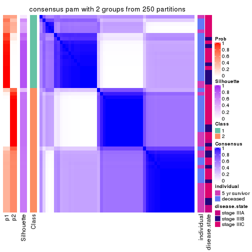
consensus_heatmap(res, k = 3)
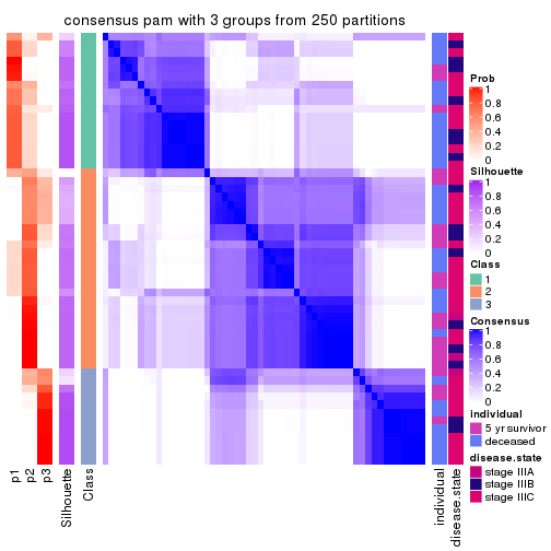
consensus_heatmap(res, k = 4)
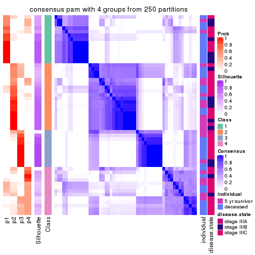
consensus_heatmap(res, k = 5)
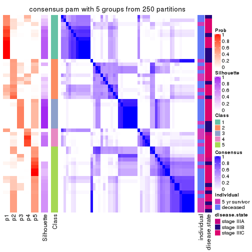
consensus_heatmap(res, k = 6)
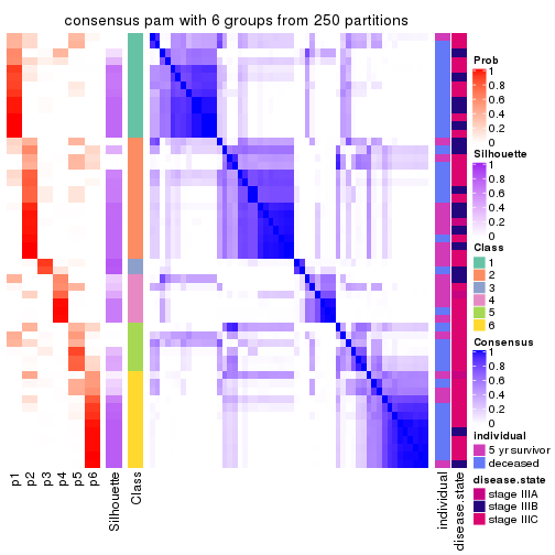
Heatmaps for the membership of samples in all partitions to see how consistent they are:
membership_heatmap(res, k = 2)
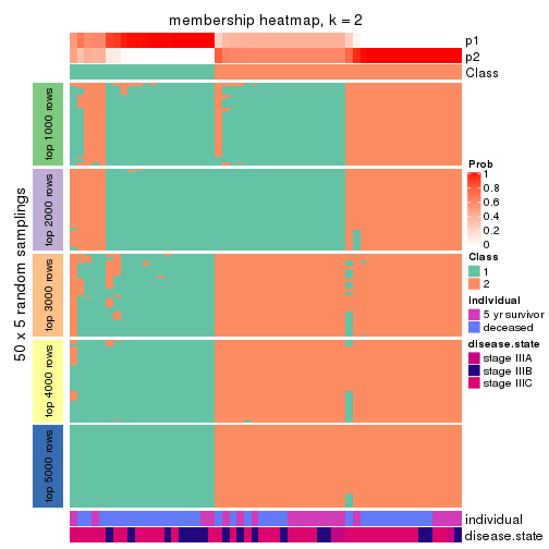
membership_heatmap(res, k = 3)
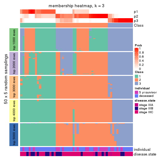
membership_heatmap(res, k = 4)
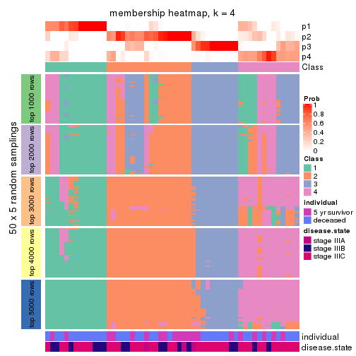
membership_heatmap(res, k = 5)
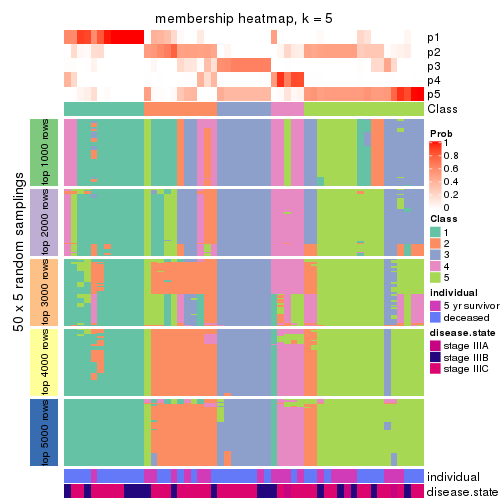
membership_heatmap(res, k = 6)
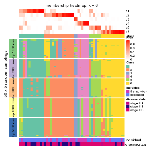
As soon as we have had the classes for columns, we can look for signatures which are significantly different between classes which can be candidate marks for certain classes. Following are the heatmaps for signatures.
Signature heatmaps where rows are scaled:
get_signatures(res, k = 2)
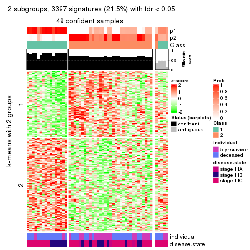
get_signatures(res, k = 3)
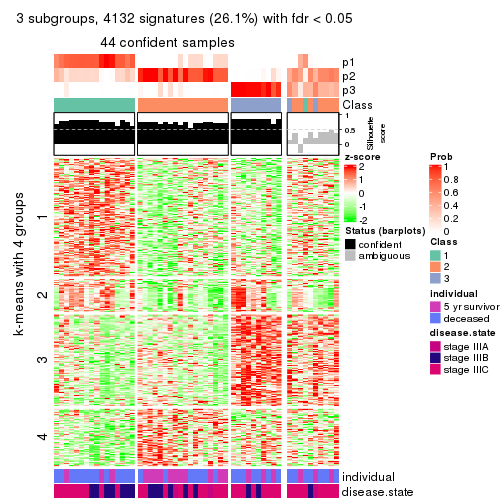
get_signatures(res, k = 4)
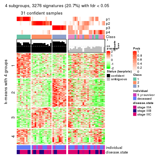
get_signatures(res, k = 5)
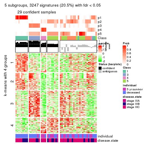
get_signatures(res, k = 6)
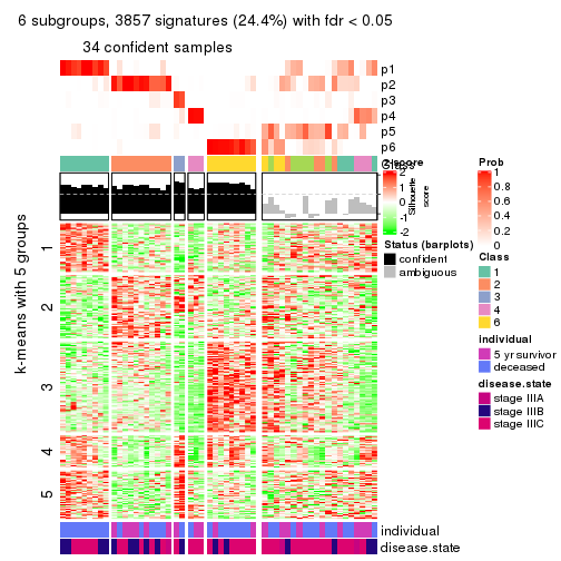
Signature heatmaps where rows are not scaled:
get_signatures(res, k = 2, scale_rows = FALSE)
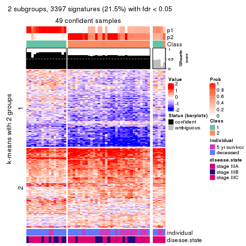
get_signatures(res, k = 3, scale_rows = FALSE)
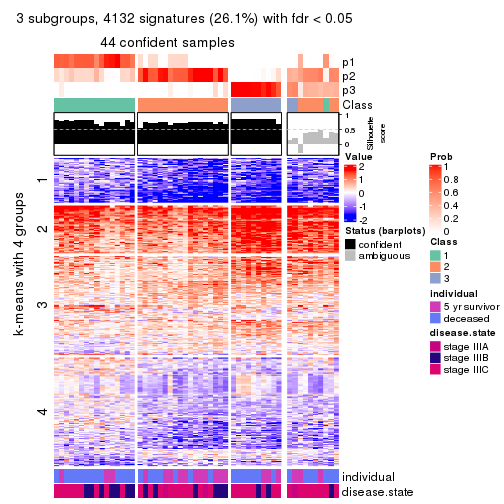
get_signatures(res, k = 4, scale_rows = FALSE)
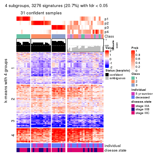
get_signatures(res, k = 5, scale_rows = FALSE)
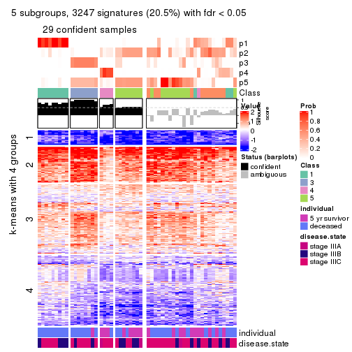
get_signatures(res, k = 6, scale_rows = FALSE)
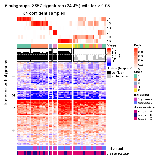
Compare the overlap of signatures from different k:
compare_signatures(res)
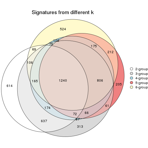
get_signature() returns a data frame invisibly. TO get the list of signatures, the function
call should be assigned to a variable explicitly. In following code, if plot argument is set
to FALSE, no heatmap is plotted while only the differential analysis is performed.
# code only for demonstration
tb = get_signature(res, k = ..., plot = FALSE)
An example of the output of tb is:
#>   which_row         fdr    mean_1    mean_2 scaled_mean_1 scaled_mean_2 km
#> 1        38 0.042760348  8.373488  9.131774    -0.5533452     0.5164555  1
#> 2        40 0.018707592  7.106213  8.469186    -0.6173731     0.5762149  1
#> 3        55 0.019134737 10.221463 11.207825    -0.6159697     0.5749050  1
#> 4        59 0.006059896  5.921854  7.869574    -0.6899429     0.6439467  1
#> 5        60 0.018055526  8.928898 10.211722    -0.6204761     0.5791110  1
#> 6        98 0.009384629 15.714769 14.887706     0.6635654    -0.6193277  2
...
The columns in tb are:
which_row: row indices corresponding to the input matrix.fdr: FDR for the differential test. mean_x: The mean value in group x.scaled_mean_x: The mean value in group x after rows are scaled.km: Row groups if k-means clustering is applied to rows.UMAP plot which shows how samples are separated.
dimension_reduction(res, k = 2, method = "UMAP")
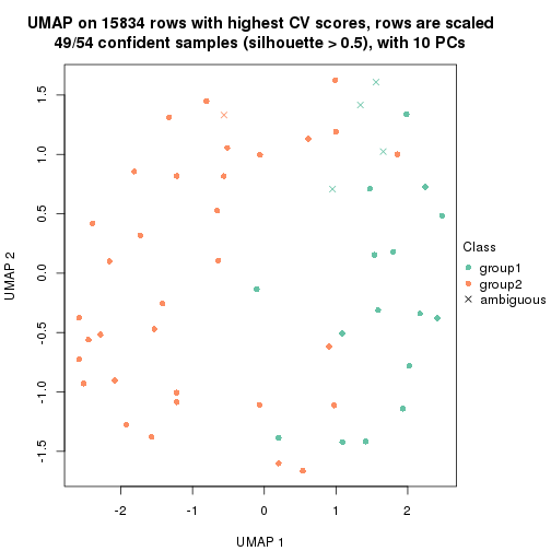
dimension_reduction(res, k = 3, method = "UMAP")
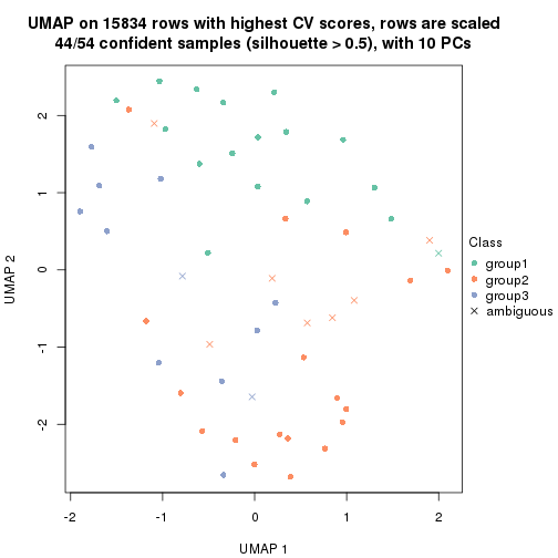
dimension_reduction(res, k = 4, method = "UMAP")
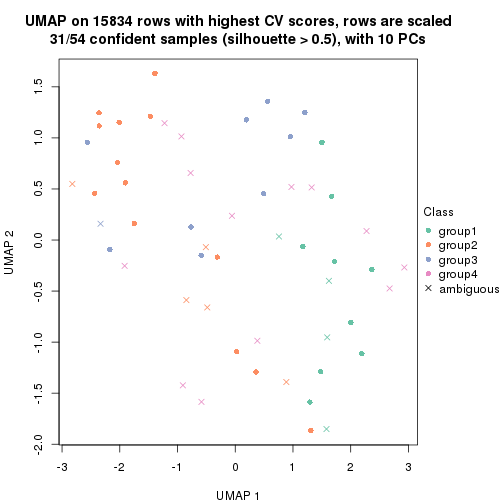
dimension_reduction(res, k = 5, method = "UMAP")
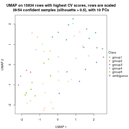
dimension_reduction(res, k = 6, method = "UMAP")
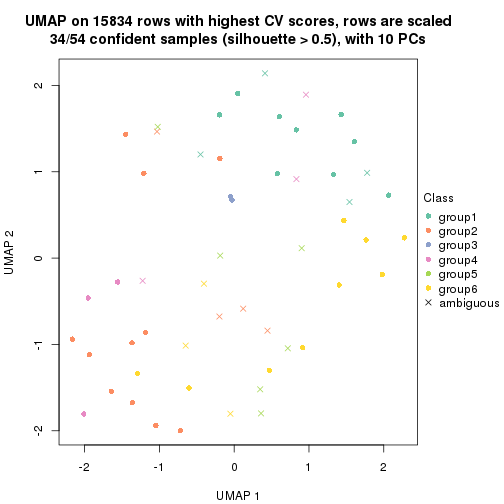
Following heatmap shows how subgroups are split when increasing k:
collect_classes(res)
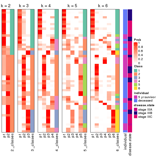
Test correlation between subgroups and known annotations. If the known annotation is numeric, one-way ANOVA test is applied, and if the known annotation is discrete, chi-squared contingency table test is applied.
test_to_known_factors(res)
#>         n individual(p) disease.state(p) k
#> CV:pam 49       0.03282            0.294 2
#> CV:pam 44       0.03307            0.326 3
#> CV:pam 31       0.00744            0.357 4
#> CV:pam 29       0.00547            0.319 5
#> CV:pam 34       0.05864            0.658 6
If matrix rows can be associated to genes, consider to use functional_enrichment(res,
...) to perform function enrichment for the signature genes. See this vignette for more detailed explanations.
The object with results only for a single top-value method and a single partition method can be extracted as:
res = res_list["CV", "mclust"]
# you can also extract it by
# res = res_list["CV:mclust"]
A summary of res and all the functions that can be applied to it:
res
#> A 'ConsensusPartition' object with k = 2, 3, 4, 5, 6.
#>   On a matrix with 15834 rows and 54 columns.
#>   Top rows (1000, 2000, 3000, 4000, 5000) are extracted by 'CV' method.
#>   Subgroups are detected by 'mclust' method.
#>   Performed in total 1250 partitions by row resampling.
#>   Best k for subgroups seems to be 6.
#>
#> Following methods can be applied to this 'ConsensusPartition' object:
#>  [1] "cola_report"             "collect_classes"         "collect_plots"
#>  [4] "collect_stats"           "colnames"                "compare_signatures"
#>  [7] "consensus_heatmap"       "dimension_reduction"     "functional_enrichment"
#> [10] "get_anno_col"            "get_anno"                "get_classes"
#> [13] "get_consensus"           "get_matrix"              "get_membership"
#> [16] "get_param"               "get_signatures"          "get_stats"
#> [19] "is_best_k"               "is_stable_k"             "membership_heatmap"
#> [22] "ncol"                    "nrow"                    "plot_ecdf"
#> [25] "rownames"                "select_partition_number" "show"
#> [28] "suggest_best_k"          "test_to_known_factors"
collect_plots() function collects all the plots made from res for all k (number of partitions)
into one single page to provide an easy and fast comparison between different k.
collect_plots(res)
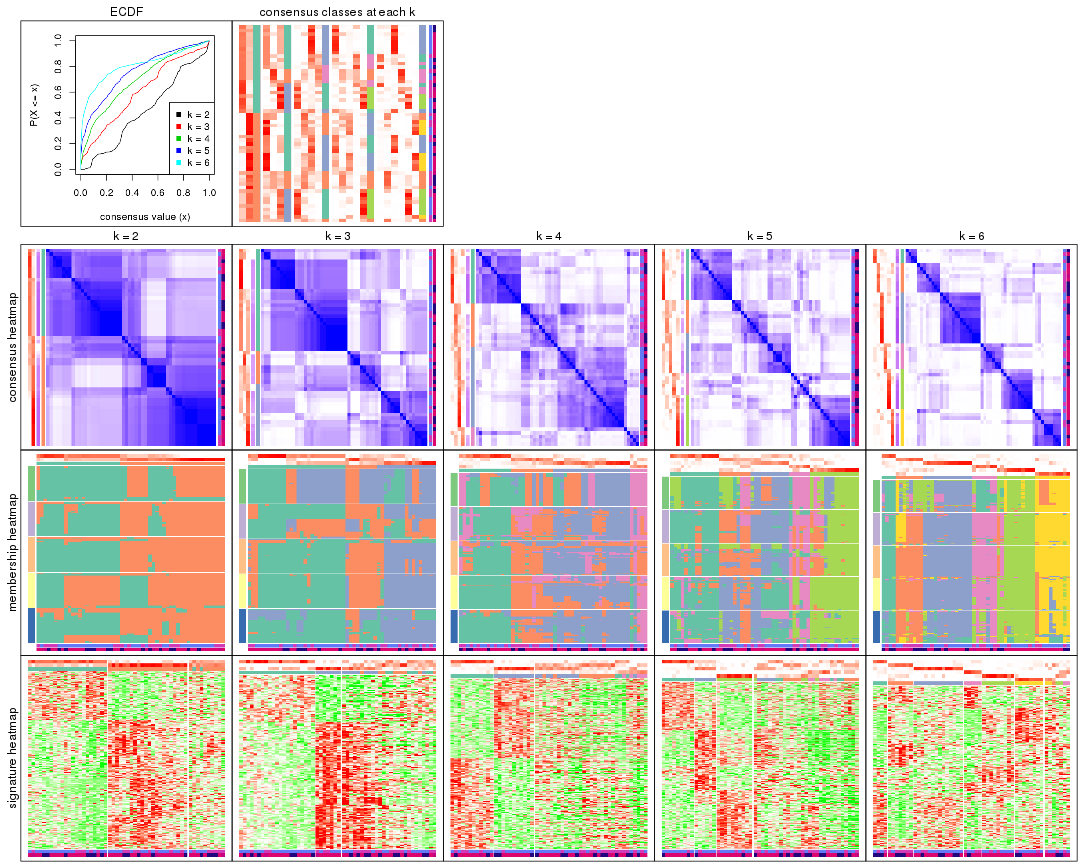
The plots are:
k and the heatmap of
predicted classes for each k.k.k.k.All the plots in panels can be made by individual functions and they are plotted later in this section.
select_partition_number() produces several plots showing different
statistics for choosing “optimized” k. There are following statistics:
k;k, the area increased is defined as \(A_k - A_{k-1}\).The detailed explanations of these statistics can be found in the cola vignette.
Generally speaking, lower PAC score, higher mean silhouette score or higher
concordance corresponds to better partition. Rand index and Jaccard index
measure how similar the current partition is compared to partition with k-1.
If they are too similar, we won't accept k is better than k-1.
select_partition_number(res)
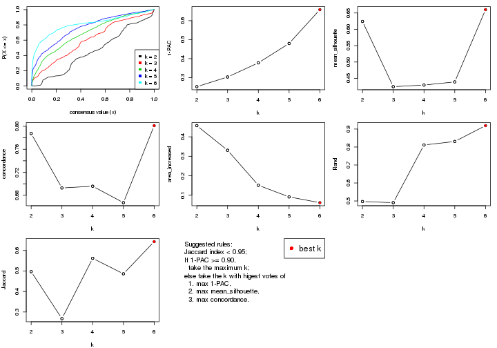
The numeric values for all these statistics can be obtained by get_stats().
get_stats(res)
#>   k 1-PAC mean_silhouette concordance area_increased  Rand Jaccard
#> 2 2 0.253           0.624       0.787         0.4575 0.497   0.497
#> 3 3 0.304           0.425       0.693         0.3308 0.491   0.267
#> 4 4 0.378           0.430       0.696         0.1508 0.811   0.562
#> 5 5 0.480           0.439       0.667         0.0910 0.831   0.486
#> 6 6 0.658           0.660       0.801         0.0615 0.919   0.643
suggest_best_k() suggests the best \(k\) based on these statistics. The rules are as follows:
suggest_best_k(res)
#> [1] 6
Following shows the table of the partitions (You need to click the show/hide
code output link to see it). The membership matrix (columns with name p*)
is inferred by
clue::cl_consensus()
function with the SE method. Basically the value in the membership matrix
represents the probability to belong to a certain group. The finall class
label for an item is determined with the group with highest probability it
belongs to.
In get_classes() function, the entropy is calculated from the membership
matrix and the silhouette score is calculated from the consensus matrix.
cbind(get_classes(res, k = 2), get_membership(res, k = 2))
#>           class entropy silhouette    p1    p2
#> GSM311939     2  0.0938      0.744 0.012 0.988
#> GSM311963     2  0.9866     -0.196 0.432 0.568
#> GSM311973     1  0.3274      0.661 0.940 0.060
#> GSM311940     2  0.5519      0.647 0.128 0.872
#> GSM311953     2  0.7745      0.563 0.228 0.772
#> GSM311974     2  0.9833      0.472 0.424 0.576
#> GSM311975     2  0.9815     -0.177 0.420 0.580
#> GSM311977     2  0.8955      0.279 0.312 0.688
#> GSM311982     1  0.3733      0.669 0.928 0.072
#> GSM311990     2  0.8016      0.619 0.244 0.756
#> GSM311943     2  0.4431      0.683 0.092 0.908
#> GSM311944     1  0.9170      0.264 0.668 0.332
#> GSM311946     2  0.9580      0.126 0.380 0.620
#> GSM311956     1  0.5178      0.654 0.884 0.116
#> GSM311967     2  0.0938      0.744 0.012 0.988
#> GSM311968     2  0.8267      0.612 0.260 0.740
#> GSM311972     1  0.8861      0.795 0.696 0.304
#> GSM311980     1  0.3733      0.669 0.928 0.072
#> GSM311981     1  0.8861      0.795 0.696 0.304
#> GSM311988     2  0.0938      0.744 0.012 0.988
#> GSM311957     2  0.0938      0.742 0.012 0.988
#> GSM311960     1  0.5178      0.654 0.884 0.116
#> GSM311971     1  0.8813      0.794 0.700 0.300
#> GSM311976     1  0.8861      0.795 0.696 0.304
#> GSM311978     1  0.9000      0.790 0.684 0.316
#> GSM311979     1  0.8909      0.794 0.692 0.308
#> GSM311983     1  0.9970      0.436 0.532 0.468
#> GSM311986     2  0.0000      0.742 0.000 1.000
#> GSM311991     1  0.8861      0.795 0.696 0.304
#> GSM311938     2  0.0938      0.744 0.012 0.988
#> GSM311941     2  0.0000      0.742 0.000 1.000
#> GSM311942     2  0.8016      0.619 0.244 0.756
#> GSM311945     1  0.5294      0.652 0.880 0.120
#> GSM311947     2  0.8016      0.619 0.244 0.756
#> GSM311948     2  0.9881      0.467 0.436 0.564
#> GSM311949     1  0.8861      0.795 0.696 0.304
#> GSM311950     2  0.0938      0.744 0.012 0.988
#> GSM311951     2  0.8016      0.619 0.244 0.756
#> GSM311952     1  0.9129      0.765 0.672 0.328
#> GSM311954     2  0.0938      0.744 0.012 0.988
#> GSM311955     2  0.9522      0.161 0.372 0.628
#> GSM311958     1  0.9323      0.727 0.652 0.348
#> GSM311959     2  0.1633      0.729 0.024 0.976
#> GSM311961     2  0.8386      0.398 0.268 0.732
#> GSM311962     1  0.9209      0.722 0.664 0.336
#> GSM311964     1  0.8861      0.795 0.696 0.304
#> GSM311965     2  0.8267      0.612 0.260 0.740
#> GSM311966     1  0.8499      0.766 0.724 0.276
#> GSM311969     2  0.1414      0.732 0.020 0.980
#> GSM311970     1  0.8861      0.795 0.696 0.304
#> GSM311984     2  0.0000      0.742 0.000 1.000
#> GSM311985     1  0.9170      0.758 0.668 0.332
#> GSM311987     2  0.0000      0.742 0.000 1.000
#> GSM311989     1  0.6712      0.598 0.824 0.176
cbind(get_classes(res, k = 3), get_membership(res, k = 3))
#>           class entropy silhouette    p1    p2    p3
#> GSM311939     1  0.0000     0.5301 1.000 0.000 0.000
#> GSM311963     2  0.9283     0.5019 0.180 0.500 0.320
#> GSM311973     3  0.0892     0.5338 0.000 0.020 0.980
#> GSM311940     2  0.9613     0.4921 0.308 0.464 0.228
#> GSM311953     2  0.9457     0.4556 0.188 0.460 0.352
#> GSM311974     3  0.7027     0.3423 0.104 0.172 0.724
#> GSM311975     1  0.6988     0.5581 0.644 0.036 0.320
#> GSM311977     2  0.9627     0.4824 0.228 0.460 0.312
#> GSM311982     3  0.5656     0.3742 0.004 0.284 0.712
#> GSM311990     3  0.6126     0.4479 0.400 0.000 0.600
#> GSM311943     1  0.5882     0.6123 0.652 0.000 0.348
#> GSM311944     3  0.0592     0.5426 0.012 0.000 0.988
#> GSM311946     3  0.9897    -0.3791 0.268 0.344 0.388
#> GSM311956     2  0.6252    -0.1514 0.000 0.556 0.444
#> GSM311967     1  0.7384    -0.0775 0.660 0.272 0.068
#> GSM311968     3  0.6208     0.5440 0.200 0.048 0.752
#> GSM311972     1  0.8345     0.4340 0.596 0.288 0.116
#> GSM311980     3  0.6299     0.1649 0.000 0.476 0.524
#> GSM311981     2  0.2173     0.4739 0.008 0.944 0.048
#> GSM311988     1  0.6280    -0.3306 0.540 0.460 0.000
#> GSM311957     1  0.6008     0.5481 0.628 0.000 0.372
#> GSM311960     3  0.3340     0.4816 0.000 0.120 0.880
#> GSM311971     1  0.6813     0.5374 0.520 0.012 0.468
#> GSM311976     3  0.9888    -0.3620 0.264 0.348 0.388
#> GSM311978     1  0.6617     0.6090 0.600 0.012 0.388
#> GSM311979     1  0.9106     0.3848 0.536 0.284 0.180
#> GSM311983     1  0.6126     0.6141 0.600 0.000 0.400
#> GSM311986     1  0.0000     0.5301 1.000 0.000 0.000
#> GSM311991     2  0.2173     0.4739 0.008 0.944 0.048
#> GSM311938     2  0.9497     0.4738 0.332 0.468 0.200
#> GSM311941     1  0.0237     0.5287 0.996 0.000 0.004
#> GSM311942     3  0.6282     0.4565 0.384 0.004 0.612
#> GSM311945     3  0.0592     0.5367 0.000 0.012 0.988
#> GSM311947     3  0.6126     0.4479 0.400 0.000 0.600
#> GSM311948     3  0.3193     0.5385 0.100 0.004 0.896
#> GSM311949     1  0.9241     0.4215 0.456 0.156 0.388
#> GSM311950     1  0.6291    -0.3398 0.532 0.468 0.000
#> GSM311951     3  0.6033     0.4914 0.336 0.004 0.660
#> GSM311952     1  0.6126     0.6141 0.600 0.000 0.400
#> GSM311954     1  0.0747     0.5164 0.984 0.016 0.000
#> GSM311955     1  0.6126     0.6141 0.600 0.000 0.400
#> GSM311958     1  0.6126     0.6141 0.600 0.000 0.400
#> GSM311959     1  0.1031     0.5400 0.976 0.000 0.024
#> GSM311961     1  0.6079     0.6151 0.612 0.000 0.388
#> GSM311962     1  0.6126     0.6141 0.600 0.000 0.400
#> GSM311964     1  0.8607     0.4648 0.592 0.256 0.152
#> GSM311965     3  0.6109     0.5442 0.192 0.048 0.760
#> GSM311966     1  0.6126     0.6141 0.600 0.000 0.400
#> GSM311969     1  0.0892     0.5388 0.980 0.000 0.020
#> GSM311970     2  0.4075     0.4972 0.072 0.880 0.048
#> GSM311984     1  0.0000     0.5301 1.000 0.000 0.000
#> GSM311985     1  0.6126     0.6141 0.600 0.000 0.400
#> GSM311987     1  0.0237     0.5274 0.996 0.004 0.000
#> GSM311989     3  0.0592     0.5426 0.012 0.000 0.988
cbind(get_classes(res, k = 4), get_membership(res, k = 4))
#>           class entropy silhouette    p1    p2    p3    p4
#> GSM311939     2  0.6079    -0.0056 0.016 0.532 0.432 0.020
#> GSM311963     2  0.7092     0.1995 0.000 0.532 0.320 0.148
#> GSM311973     1  0.3526     0.7305 0.872 0.008 0.080 0.040
#> GSM311940     2  0.8161     0.3265 0.180 0.580 0.104 0.136
#> GSM311953     2  0.8576     0.2740 0.224 0.528 0.112 0.136
#> GSM311974     1  0.7528     0.4540 0.616 0.168 0.048 0.168
#> GSM311975     3  0.5866     0.3161 0.004 0.304 0.644 0.048
#> GSM311977     2  0.7054     0.3970 0.140 0.640 0.192 0.028
#> GSM311982     1  0.6443     0.3397 0.548 0.000 0.076 0.376
#> GSM311990     1  0.4428     0.5841 0.720 0.276 0.004 0.000
#> GSM311943     3  0.5368     0.5422 0.176 0.024 0.756 0.044
#> GSM311944     1  0.2941     0.7370 0.888 0.008 0.096 0.008
#> GSM311946     2  0.8860     0.2800 0.204 0.488 0.212 0.096
#> GSM311956     4  0.7968    -0.0738 0.384 0.152 0.024 0.440
#> GSM311967     2  0.7051     0.4274 0.096 0.680 0.108 0.116
#> GSM311968     1  0.1059     0.7417 0.972 0.012 0.016 0.000
#> GSM311972     3  0.5290     0.2630 0.004 0.004 0.552 0.440
#> GSM311980     1  0.7605    -0.0148 0.440 0.108 0.024 0.428
#> GSM311981     4  0.5697     0.4640 0.000 0.292 0.052 0.656
#> GSM311988     2  0.4801     0.4712 0.044 0.800 0.136 0.020
#> GSM311957     3  0.7357     0.3286 0.300 0.092 0.572 0.036
#> GSM311960     1  0.6744     0.5703 0.688 0.080 0.064 0.168
#> GSM311971     3  0.4762     0.5741 0.080 0.004 0.796 0.120
#> GSM311976     3  0.6297     0.1697 0.004 0.336 0.596 0.064
#> GSM311978     3  0.4401     0.5100 0.004 0.000 0.724 0.272
#> GSM311979     4  0.6237    -0.2609 0.044 0.004 0.448 0.504
#> GSM311983     3  0.1114     0.6402 0.004 0.016 0.972 0.008
#> GSM311986     3  0.6601     0.1064 0.036 0.428 0.512 0.024
#> GSM311991     4  0.6286     0.3847 0.000 0.384 0.064 0.552
#> GSM311938     2  0.5711     0.4459 0.040 0.652 0.304 0.004
#> GSM311941     3  0.6976     0.3177 0.044 0.332 0.576 0.048
#> GSM311942     1  0.3982     0.6243 0.776 0.220 0.004 0.000
#> GSM311945     1  0.2658     0.7400 0.904 0.004 0.080 0.012
#> GSM311947     1  0.4072     0.6067 0.748 0.252 0.000 0.000
#> GSM311948     1  0.3641     0.7387 0.868 0.052 0.072 0.008
#> GSM311949     3  0.4955     0.4243 0.004 0.244 0.728 0.024
#> GSM311950     2  0.5799     0.4098 0.040 0.752 0.072 0.136
#> GSM311951     1  0.1854     0.7408 0.940 0.048 0.012 0.000
#> GSM311952     3  0.1576     0.6375 0.004 0.000 0.948 0.048
#> GSM311954     2  0.6034     0.0612 0.016 0.556 0.408 0.020
#> GSM311955     3  0.3997     0.5884 0.120 0.028 0.840 0.012
#> GSM311958     3  0.0469     0.6397 0.000 0.012 0.988 0.000
#> GSM311959     3  0.6064     0.4223 0.040 0.268 0.668 0.024
#> GSM311961     3  0.2222     0.6199 0.000 0.060 0.924 0.016
#> GSM311962     3  0.0927     0.6401 0.000 0.016 0.976 0.008
#> GSM311964     3  0.7319     0.3083 0.004 0.156 0.524 0.316
#> GSM311965     1  0.1406     0.7435 0.960 0.016 0.024 0.000
#> GSM311966     3  0.1674     0.6380 0.004 0.012 0.952 0.032
#> GSM311969     3  0.6307     0.4527 0.040 0.252 0.668 0.040
#> GSM311970     4  0.6293     0.4389 0.016 0.316 0.048 0.620
#> GSM311984     3  0.6090     0.1441 0.016 0.440 0.524 0.020
#> GSM311985     3  0.2382     0.6302 0.004 0.004 0.912 0.080
#> GSM311987     2  0.6524    -0.0279 0.036 0.504 0.440 0.020
#> GSM311989     1  0.2983     0.7312 0.880 0.004 0.108 0.008
cbind(get_classes(res, k = 5), get_membership(res, k = 5))
#>           class entropy silhouette    p1    p2    p3    p4    p5
#> GSM311939     3  0.6083     0.5987 0.232 0.176 0.588 0.000 0.004
#> GSM311963     2  0.7397     0.3511 0.236 0.480 0.244 0.012 0.028
#> GSM311973     5  0.5528     0.4522 0.016 0.256 0.000 0.076 0.652
#> GSM311940     2  0.5651     0.4717 0.000 0.636 0.124 0.004 0.236
#> GSM311953     2  0.5666     0.4732 0.012 0.624 0.084 0.000 0.280
#> GSM311974     5  0.4169     0.5164 0.000 0.240 0.000 0.028 0.732
#> GSM311975     1  0.6038     0.5306 0.680 0.172 0.096 0.012 0.040
#> GSM311977     2  0.6648     0.4847 0.040 0.612 0.124 0.012 0.212
#> GSM311982     4  0.5501     0.2177 0.068 0.000 0.008 0.612 0.312
#> GSM311990     5  0.4597     0.3096 0.000 0.012 0.424 0.000 0.564
#> GSM311943     1  0.5532     0.4646 0.668 0.000 0.092 0.016 0.224
#> GSM311944     5  0.1764     0.6989 0.064 0.000 0.008 0.000 0.928
#> GSM311946     2  0.6205     0.4071 0.084 0.576 0.032 0.000 0.308
#> GSM311956     4  0.7505    -0.0730 0.000 0.272 0.036 0.356 0.336
#> GSM311967     3  0.5361     0.1626 0.004 0.436 0.516 0.000 0.044
#> GSM311968     5  0.0290     0.7306 0.000 0.000 0.008 0.000 0.992
#> GSM311972     4  0.5099     0.4473 0.180 0.056 0.028 0.732 0.004
#> GSM311980     5  0.7506    -0.1086 0.000 0.276 0.036 0.324 0.364
#> GSM311981     2  0.6843     0.1296 0.016 0.452 0.180 0.352 0.000
#> GSM311988     3  0.7622     0.0922 0.076 0.344 0.432 0.004 0.144
#> GSM311957     1  0.6535     0.2743 0.532 0.004 0.128 0.016 0.320
#> GSM311960     5  0.6004     0.3443 0.000 0.256 0.000 0.168 0.576
#> GSM311971     1  0.5004     0.3472 0.656 0.024 0.008 0.304 0.008
#> GSM311976     1  0.6610     0.2960 0.560 0.300 0.104 0.024 0.012
#> GSM311978     4  0.5033    -0.0192 0.444 0.012 0.008 0.532 0.004
#> GSM311979     4  0.2753     0.4492 0.136 0.000 0.008 0.856 0.000
#> GSM311983     1  0.1041     0.7023 0.964 0.000 0.032 0.000 0.004
#> GSM311986     3  0.4109     0.6188 0.260 0.008 0.724 0.008 0.000
#> GSM311991     2  0.7201     0.1131 0.032 0.420 0.192 0.356 0.000
#> GSM311938     2  0.7978    -0.0843 0.164 0.380 0.352 0.004 0.100
#> GSM311941     3  0.5422     0.5632 0.312 0.004 0.628 0.016 0.040
#> GSM311942     5  0.2890     0.6395 0.004 0.000 0.160 0.000 0.836
#> GSM311945     5  0.0486     0.7308 0.004 0.004 0.004 0.000 0.988
#> GSM311947     5  0.4272     0.5833 0.000 0.052 0.196 0.000 0.752
#> GSM311948     5  0.1571     0.7098 0.000 0.060 0.004 0.000 0.936
#> GSM311949     1  0.6171     0.4090 0.600 0.292 0.076 0.020 0.012
#> GSM311950     3  0.5114     0.1096 0.000 0.476 0.488 0.000 0.036
#> GSM311951     5  0.0290     0.7306 0.000 0.000 0.008 0.000 0.992
#> GSM311952     1  0.2264     0.6980 0.920 0.008 0.044 0.024 0.004
#> GSM311954     3  0.5934     0.5769 0.252 0.144 0.600 0.000 0.004
#> GSM311955     1  0.3803     0.5907 0.804 0.000 0.056 0.000 0.140
#> GSM311958     1  0.1205     0.6991 0.956 0.000 0.040 0.000 0.004
#> GSM311959     3  0.5364     0.3526 0.460 0.008 0.496 0.000 0.036
#> GSM311961     1  0.2570     0.6639 0.880 0.004 0.108 0.000 0.008
#> GSM311962     1  0.0865     0.7031 0.972 0.000 0.024 0.000 0.004
#> GSM311964     4  0.7488     0.1856 0.252 0.272 0.036 0.436 0.004
#> GSM311965     5  0.0451     0.7298 0.000 0.008 0.004 0.000 0.988
#> GSM311966     1  0.1267     0.7049 0.960 0.000 0.024 0.012 0.004
#> GSM311969     3  0.5717     0.3158 0.472 0.012 0.472 0.008 0.036
#> GSM311970     2  0.6814     0.0779 0.008 0.432 0.176 0.380 0.004
#> GSM311984     3  0.5784     0.5779 0.252 0.144 0.604 0.000 0.000
#> GSM311985     1  0.3427     0.6350 0.836 0.000 0.028 0.128 0.008
#> GSM311987     3  0.4040     0.6233 0.260 0.016 0.724 0.000 0.000
#> GSM311989     5  0.1628     0.7051 0.056 0.000 0.008 0.000 0.936
cbind(get_classes(res, k = 6), get_membership(res, k = 6))
#>           class entropy silhouette    p1    p2    p3    p4    p5    p6
#> GSM311939     6  0.3580     0.7222 0.060 0.096 0.016 0.000 0.004 0.824
#> GSM311963     2  0.3465     0.5951 0.000 0.820 0.112 0.060 0.004 0.004
#> GSM311973     4  0.5928     0.1847 0.008 0.108 0.008 0.460 0.412 0.004
#> GSM311940     2  0.4383     0.7084 0.000 0.736 0.004 0.024 0.196 0.040
#> GSM311953     2  0.3549     0.7090 0.000 0.784 0.004 0.024 0.184 0.004
#> GSM311974     5  0.4334     0.3715 0.000 0.316 0.004 0.024 0.652 0.004
#> GSM311975     3  0.2882     0.8342 0.036 0.044 0.884 0.024 0.004 0.008
#> GSM311977     2  0.3956     0.7219 0.000 0.780 0.024 0.032 0.160 0.004
#> GSM311982     1  0.3150     0.7459 0.856 0.000 0.036 0.068 0.040 0.000
#> GSM311990     6  0.3673     0.5217 0.004 0.016 0.000 0.000 0.244 0.736
#> GSM311943     3  0.3773     0.7126 0.020 0.000 0.768 0.000 0.192 0.020
#> GSM311944     5  0.2095     0.7585 0.016 0.000 0.076 0.004 0.904 0.000
#> GSM311946     2  0.4783     0.6037 0.000 0.680 0.044 0.024 0.248 0.004
#> GSM311956     4  0.4472     0.6578 0.152 0.000 0.000 0.728 0.112 0.008
#> GSM311967     6  0.4051     0.0451 0.008 0.432 0.000 0.000 0.000 0.560
#> GSM311968     5  0.0146     0.8043 0.000 0.000 0.004 0.000 0.996 0.000
#> GSM311972     1  0.4204     0.6728 0.740 0.000 0.132 0.128 0.000 0.000
#> GSM311980     4  0.4990     0.6480 0.152 0.016 0.000 0.696 0.132 0.004
#> GSM311981     4  0.1823     0.6415 0.004 0.036 0.012 0.932 0.000 0.016
#> GSM311988     2  0.5442     0.5330 0.000 0.556 0.004 0.000 0.128 0.312
#> GSM311957     3  0.4821     0.5601 0.020 0.004 0.644 0.000 0.296 0.036
#> GSM311960     5  0.5958    -0.2735 0.068 0.036 0.004 0.436 0.452 0.004
#> GSM311971     3  0.4335     0.7330 0.136 0.100 0.752 0.004 0.008 0.000
#> GSM311976     3  0.3765     0.7907 0.036 0.112 0.808 0.044 0.000 0.000
#> GSM311978     1  0.4357     0.6343 0.700 0.076 0.224 0.000 0.000 0.000
#> GSM311979     1  0.2451     0.7615 0.888 0.000 0.040 0.068 0.004 0.000
#> GSM311983     3  0.0458     0.8590 0.016 0.000 0.984 0.000 0.000 0.000
#> GSM311986     6  0.1053     0.7474 0.012 0.004 0.020 0.000 0.000 0.964
#> GSM311991     4  0.1508     0.6409 0.016 0.020 0.004 0.948 0.000 0.012
#> GSM311938     2  0.6263     0.5672 0.000 0.576 0.132 0.008 0.056 0.228
#> GSM311941     6  0.1889     0.7483 0.020 0.004 0.056 0.000 0.000 0.920
#> GSM311942     5  0.2135     0.7150 0.000 0.000 0.000 0.000 0.872 0.128
#> GSM311945     5  0.0767     0.8032 0.000 0.008 0.004 0.012 0.976 0.000
#> GSM311947     5  0.4637     0.5201 0.004 0.076 0.000 0.000 0.672 0.248
#> GSM311948     5  0.1363     0.7955 0.000 0.028 0.004 0.012 0.952 0.004
#> GSM311949     3  0.3881     0.7958 0.036 0.112 0.808 0.036 0.000 0.008
#> GSM311950     2  0.3976     0.3496 0.004 0.612 0.000 0.004 0.000 0.380
#> GSM311951     5  0.0146     0.8043 0.000 0.000 0.004 0.000 0.996 0.000
#> GSM311952     3  0.1261     0.8612 0.004 0.028 0.956 0.000 0.004 0.008
#> GSM311954     6  0.3675     0.7231 0.064 0.092 0.020 0.000 0.004 0.820
#> GSM311955     3  0.2798     0.7901 0.012 0.008 0.856 0.000 0.120 0.004
#> GSM311958     3  0.0582     0.8616 0.004 0.004 0.984 0.000 0.004 0.004
#> GSM311959     6  0.4421     0.4952 0.028 0.008 0.328 0.000 0.000 0.636
#> GSM311961     3  0.1292     0.8564 0.028 0.004 0.956 0.004 0.004 0.004
#> GSM311962     3  0.0458     0.8590 0.016 0.000 0.984 0.000 0.000 0.000
#> GSM311964     4  0.5809     0.3619 0.144 0.028 0.248 0.580 0.000 0.000
#> GSM311965     5  0.0551     0.8040 0.008 0.000 0.004 0.000 0.984 0.004
#> GSM311966     3  0.0458     0.8590 0.016 0.000 0.984 0.000 0.000 0.000
#> GSM311969     6  0.3516     0.6836 0.024 0.012 0.172 0.000 0.000 0.792
#> GSM311970     4  0.2988     0.6430 0.152 0.024 0.000 0.824 0.000 0.000
#> GSM311984     6  0.3756     0.7231 0.064 0.092 0.024 0.000 0.004 0.816
#> GSM311985     3  0.1141     0.8512 0.052 0.000 0.948 0.000 0.000 0.000
#> GSM311987     6  0.1806     0.7516 0.020 0.008 0.044 0.000 0.000 0.928
#> GSM311989     5  0.1929     0.7812 0.016 0.008 0.048 0.004 0.924 0.000
Heatmaps for the consensus matrix. It visualizes the probability of two samples to be in a same group.
consensus_heatmap(res, k = 2)
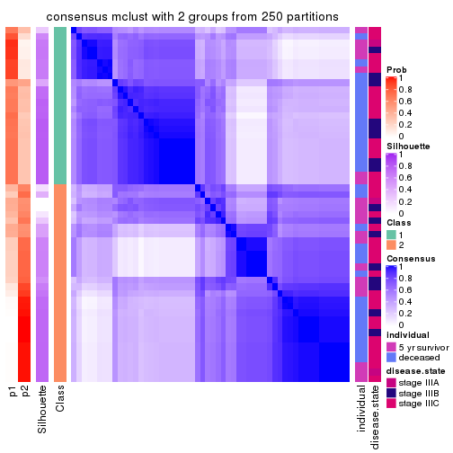
consensus_heatmap(res, k = 3)
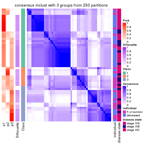
consensus_heatmap(res, k = 4)
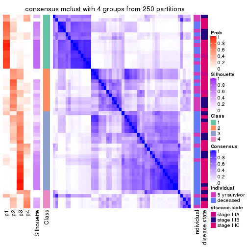
consensus_heatmap(res, k = 5)
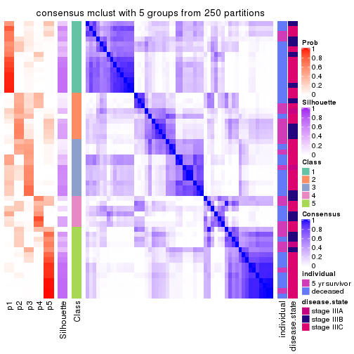
consensus_heatmap(res, k = 6)
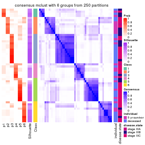
Heatmaps for the membership of samples in all partitions to see how consistent they are:
membership_heatmap(res, k = 2)
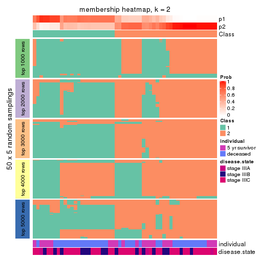
membership_heatmap(res, k = 3)
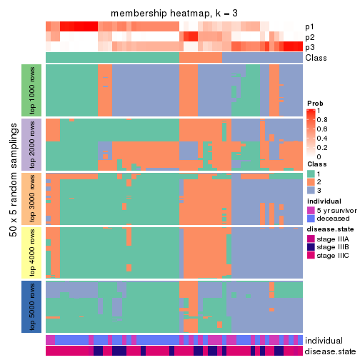
membership_heatmap(res, k = 4)
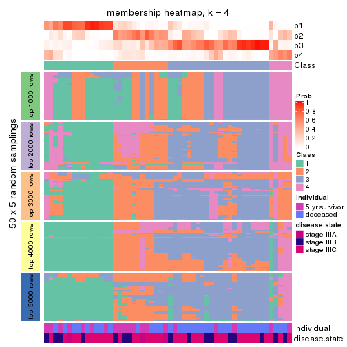
membership_heatmap(res, k = 5)
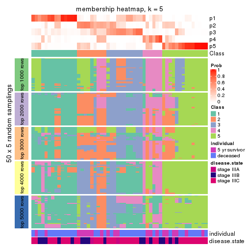
membership_heatmap(res, k = 6)
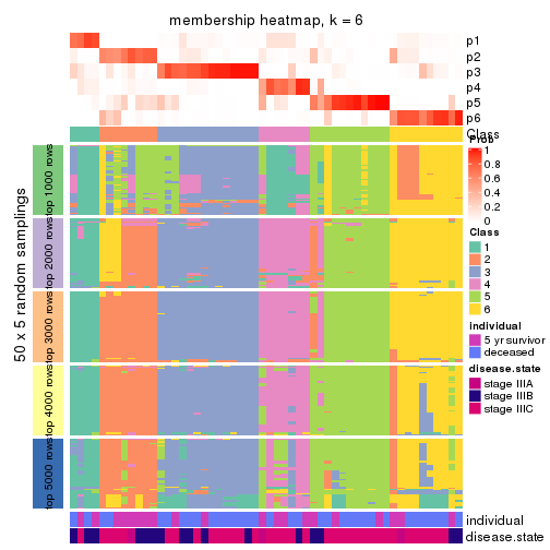
As soon as we have had the classes for columns, we can look for signatures which are significantly different between classes which can be candidate marks for certain classes. Following are the heatmaps for signatures.
Signature heatmaps where rows are scaled:
get_signatures(res, k = 2)
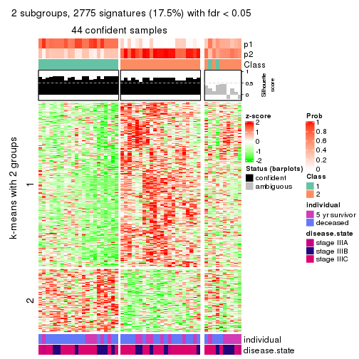
get_signatures(res, k = 3)
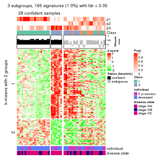
get_signatures(res, k = 4)
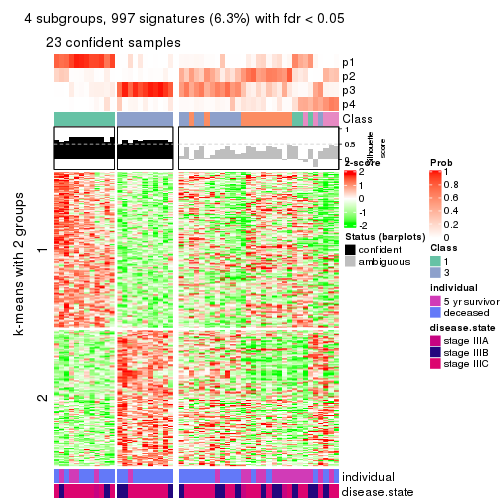
get_signatures(res, k = 5)
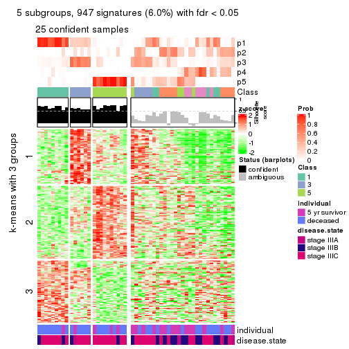
get_signatures(res, k = 6)
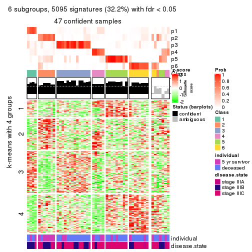
Signature heatmaps where rows are not scaled:
get_signatures(res, k = 2, scale_rows = FALSE)
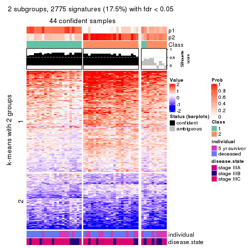
get_signatures(res, k = 3, scale_rows = FALSE)
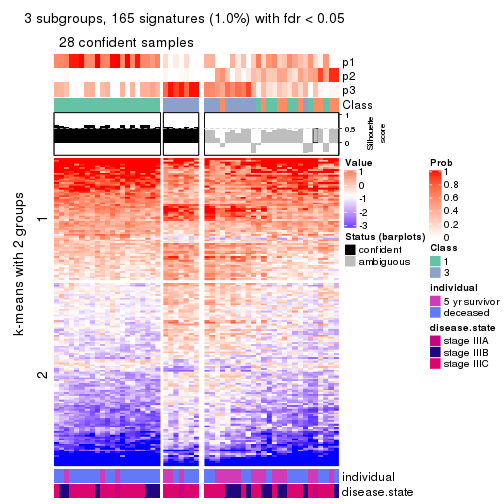
get_signatures(res, k = 4, scale_rows = FALSE)
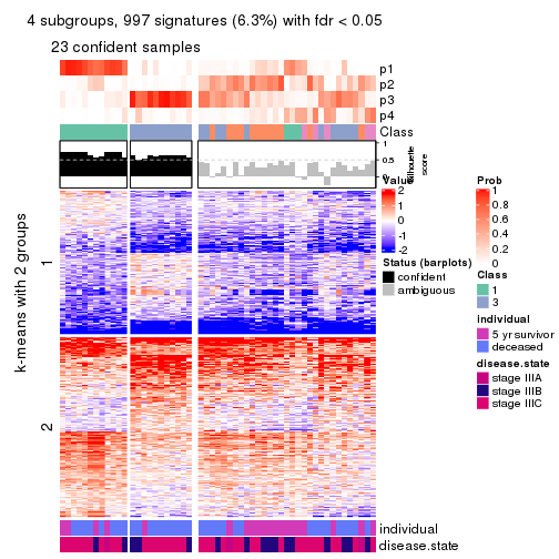
get_signatures(res, k = 5, scale_rows = FALSE)
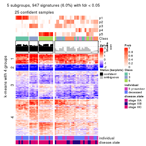
get_signatures(res, k = 6, scale_rows = FALSE)
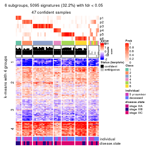
Compare the overlap of signatures from different k:
compare_signatures(res)
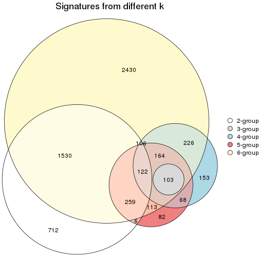
get_signature() returns a data frame invisibly. TO get the list of signatures, the function
call should be assigned to a variable explicitly. In following code, if plot argument is set
to FALSE, no heatmap is plotted while only the differential analysis is performed.
# code only for demonstration
tb = get_signature(res, k = ..., plot = FALSE)
An example of the output of tb is:
#>   which_row         fdr    mean_1    mean_2 scaled_mean_1 scaled_mean_2 km
#> 1        38 0.042760348  8.373488  9.131774    -0.5533452     0.5164555  1
#> 2        40 0.018707592  7.106213  8.469186    -0.6173731     0.5762149  1
#> 3        55 0.019134737 10.221463 11.207825    -0.6159697     0.5749050  1
#> 4        59 0.006059896  5.921854  7.869574    -0.6899429     0.6439467  1
#> 5        60 0.018055526  8.928898 10.211722    -0.6204761     0.5791110  1
#> 6        98 0.009384629 15.714769 14.887706     0.6635654    -0.6193277  2
...
The columns in tb are:
which_row: row indices corresponding to the input matrix.fdr: FDR for the differential test. mean_x: The mean value in group x.scaled_mean_x: The mean value in group x after rows are scaled.km: Row groups if k-means clustering is applied to rows.UMAP plot which shows how samples are separated.
dimension_reduction(res, k = 2, method = "UMAP")
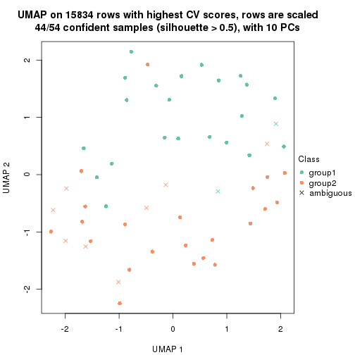
dimension_reduction(res, k = 3, method = "UMAP")
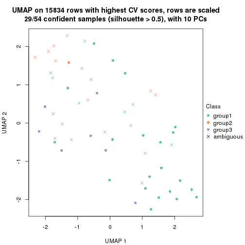
dimension_reduction(res, k = 4, method = "UMAP")
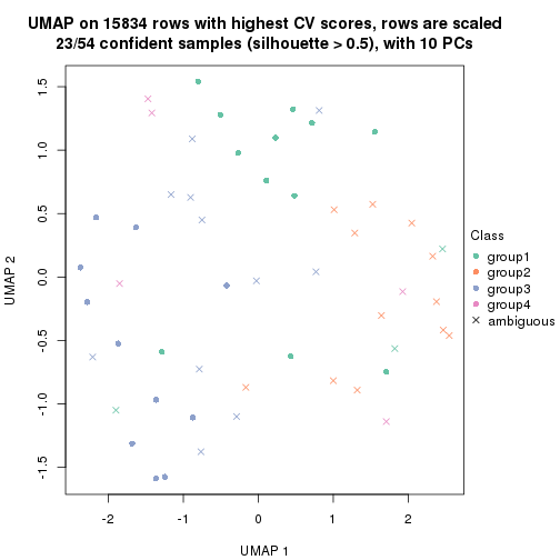
dimension_reduction(res, k = 5, method = "UMAP")
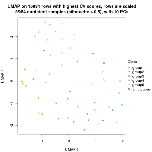
dimension_reduction(res, k = 6, method = "UMAP")
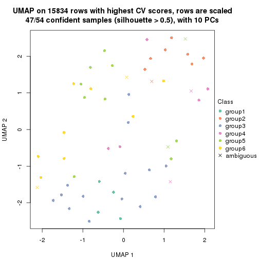
Following heatmap shows how subgroups are split when increasing k:
collect_classes(res)

Test correlation between subgroups and known annotations. If the known annotation is numeric, one-way ANOVA test is applied, and if the known annotation is discrete, chi-squared contingency table test is applied.
test_to_known_factors(res)
#>            n individual(p) disease.state(p) k
#> CV:mclust 44        0.7462            0.792 2
#> CV:mclust 29        0.0609            0.019 3
#> CV:mclust 23        0.3671            0.544 4
#> CV:mclust 25        0.5738            0.423 5
#> CV:mclust 47        0.0225            0.180 6
If matrix rows can be associated to genes, consider to use functional_enrichment(res,
...) to perform function enrichment for the signature genes. See this vignette for more detailed explanations.
The object with results only for a single top-value method and a single partition method can be extracted as:
res = res_list["CV", "NMF"]
# you can also extract it by
# res = res_list["CV:NMF"]
A summary of res and all the functions that can be applied to it:
res
#> A 'ConsensusPartition' object with k = 2, 3, 4, 5, 6.
#>   On a matrix with 15834 rows and 54 columns.
#>   Top rows (1000, 2000, 3000, 4000, 5000) are extracted by 'CV' method.
#>   Subgroups are detected by 'NMF' method.
#>   Performed in total 1250 partitions by row resampling.
#>   Best k for subgroups seems to be 2.
#>
#> Following methods can be applied to this 'ConsensusPartition' object:
#>  [1] "cola_report"             "collect_classes"         "collect_plots"
#>  [4] "collect_stats"           "colnames"                "compare_signatures"
#>  [7] "consensus_heatmap"       "dimension_reduction"     "functional_enrichment"
#> [10] "get_anno_col"            "get_anno"                "get_classes"
#> [13] "get_consensus"           "get_matrix"              "get_membership"
#> [16] "get_param"               "get_signatures"          "get_stats"
#> [19] "is_best_k"               "is_stable_k"             "membership_heatmap"
#> [22] "ncol"                    "nrow"                    "plot_ecdf"
#> [25] "rownames"                "select_partition_number" "show"
#> [28] "suggest_best_k"          "test_to_known_factors"
collect_plots() function collects all the plots made from res for all k (number of partitions)
into one single page to provide an easy and fast comparison between different k.
collect_plots(res)
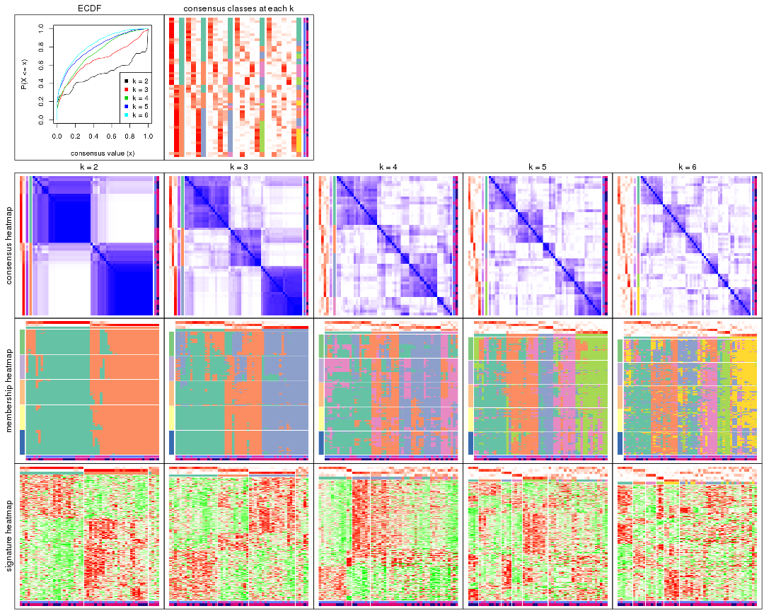
The plots are:
k and the heatmap of
predicted classes for each k.k.k.k.All the plots in panels can be made by individual functions and they are plotted later in this section.
select_partition_number() produces several plots showing different
statistics for choosing “optimized” k. There are following statistics:
k;k, the area increased is defined as \(A_k - A_{k-1}\).The detailed explanations of these statistics can be found in the cola vignette.
Generally speaking, lower PAC score, higher mean silhouette score or higher
concordance corresponds to better partition. Rand index and Jaccard index
measure how similar the current partition is compared to partition with k-1.
If they are too similar, we won't accept k is better than k-1.
select_partition_number(res)
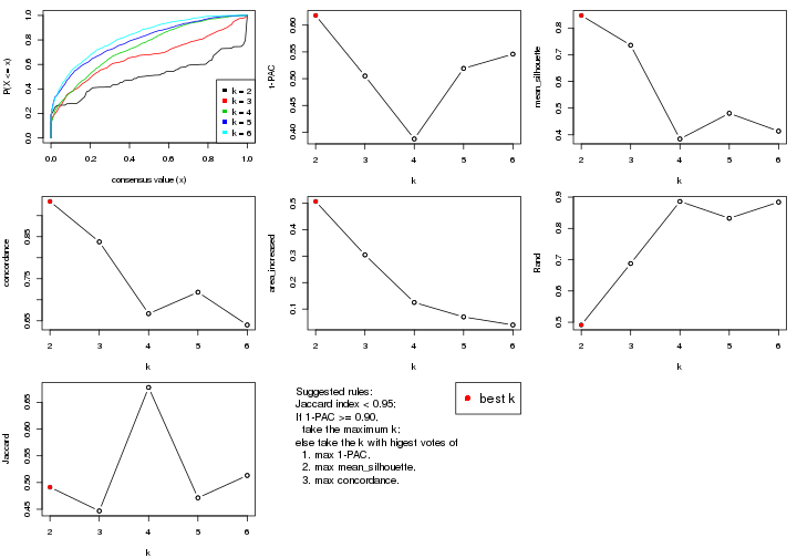
The numeric values for all these statistics can be obtained by get_stats().
get_stats(res)
#>   k 1-PAC mean_silhouette concordance area_increased  Rand Jaccard
#> 2 2 0.618           0.847       0.934         0.5064 0.491   0.491
#> 3 3 0.505           0.736       0.838         0.3046 0.688   0.447
#> 4 4 0.387           0.384       0.667         0.1250 0.886   0.678
#> 5 5 0.519           0.480       0.718         0.0703 0.832   0.471
#> 6 6 0.546           0.414       0.640         0.0400 0.884   0.513
suggest_best_k() suggests the best \(k\) based on these statistics. The rules are as follows:
suggest_best_k(res)
#> [1] 2
Following shows the table of the partitions (You need to click the show/hide
code output link to see it). The membership matrix (columns with name p*)
is inferred by
clue::cl_consensus()
function with the SE method. Basically the value in the membership matrix
represents the probability to belong to a certain group. The finall class
label for an item is determined with the group with highest probability it
belongs to.
In get_classes() function, the entropy is calculated from the membership
matrix and the silhouette score is calculated from the consensus matrix.
cbind(get_classes(res, k = 2), get_membership(res, k = 2))
#>           class entropy silhouette    p1    p2
#> GSM311939     2  0.0000      0.917 0.000 1.000
#> GSM311963     2  0.9491      0.446 0.368 0.632
#> GSM311973     1  0.0000      0.928 1.000 0.000
#> GSM311940     2  0.0000      0.917 0.000 1.000
#> GSM311953     2  0.6712      0.759 0.176 0.824
#> GSM311974     2  0.0000      0.917 0.000 1.000
#> GSM311975     1  0.6343      0.784 0.840 0.160
#> GSM311977     2  0.4022      0.863 0.080 0.920
#> GSM311982     1  0.0000      0.928 1.000 0.000
#> GSM311990     2  0.0000      0.917 0.000 1.000
#> GSM311943     2  0.6623      0.765 0.172 0.828
#> GSM311944     1  0.7376      0.741 0.792 0.208
#> GSM311946     2  0.9795      0.327 0.416 0.584
#> GSM311956     1  0.0000      0.928 1.000 0.000
#> GSM311967     2  0.0000      0.917 0.000 1.000
#> GSM311968     2  0.5842      0.804 0.140 0.860
#> GSM311972     1  0.0000      0.928 1.000 0.000
#> GSM311980     1  0.0000      0.928 1.000 0.000
#> GSM311981     1  0.0000      0.928 1.000 0.000
#> GSM311988     2  0.0000      0.917 0.000 1.000
#> GSM311957     2  0.0938      0.911 0.012 0.988
#> GSM311960     1  0.6712      0.778 0.824 0.176
#> GSM311971     1  0.0000      0.928 1.000 0.000
#> GSM311976     1  0.0000      0.928 1.000 0.000
#> GSM311978     1  0.0000      0.928 1.000 0.000
#> GSM311979     1  0.0000      0.928 1.000 0.000
#> GSM311983     1  0.6048      0.807 0.852 0.148
#> GSM311986     2  0.0000      0.917 0.000 1.000
#> GSM311991     1  0.0000      0.928 1.000 0.000
#> GSM311938     2  0.0672      0.914 0.008 0.992
#> GSM311941     2  0.0000      0.917 0.000 1.000
#> GSM311942     2  0.0000      0.917 0.000 1.000
#> GSM311945     1  0.7219      0.749 0.800 0.200
#> GSM311947     2  0.0000      0.917 0.000 1.000
#> GSM311948     2  0.1633      0.904 0.024 0.976
#> GSM311949     1  0.0000      0.928 1.000 0.000
#> GSM311950     2  0.0000      0.917 0.000 1.000
#> GSM311951     2  0.0000      0.917 0.000 1.000
#> GSM311952     1  0.1184      0.920 0.984 0.016
#> GSM311954     2  0.0000      0.917 0.000 1.000
#> GSM311955     2  0.9896      0.158 0.440 0.560
#> GSM311958     1  0.0938      0.922 0.988 0.012
#> GSM311959     2  0.0000      0.917 0.000 1.000
#> GSM311961     1  0.8861      0.543 0.696 0.304
#> GSM311962     1  0.0672      0.924 0.992 0.008
#> GSM311964     1  0.0000      0.928 1.000 0.000
#> GSM311965     2  0.6438      0.776 0.164 0.836
#> GSM311966     1  0.0000      0.928 1.000 0.000
#> GSM311969     2  0.0000      0.917 0.000 1.000
#> GSM311970     1  0.0000      0.928 1.000 0.000
#> GSM311984     2  0.0000      0.917 0.000 1.000
#> GSM311985     1  0.0000      0.928 1.000 0.000
#> GSM311987     2  0.0000      0.917 0.000 1.000
#> GSM311989     1  0.9323      0.498 0.652 0.348
cbind(get_classes(res, k = 3), get_membership(res, k = 3))
#>           class entropy silhouette    p1    p2    p3
#> GSM311939     3  0.3276     0.8820 0.068 0.024 0.908
#> GSM311963     3  0.8571     0.4310 0.272 0.140 0.588
#> GSM311973     2  0.2261     0.7327 0.068 0.932 0.000
#> GSM311940     2  0.6079     0.4812 0.000 0.612 0.388
#> GSM311953     2  0.6710     0.6967 0.072 0.732 0.196
#> GSM311974     2  0.5465     0.6195 0.000 0.712 0.288
#> GSM311975     2  0.6820     0.6412 0.248 0.700 0.052
#> GSM311977     2  0.7129     0.6833 0.104 0.716 0.180
#> GSM311982     1  0.5497     0.6857 0.708 0.292 0.000
#> GSM311990     3  0.0237     0.9011 0.000 0.004 0.996
#> GSM311943     1  0.6045     0.4673 0.620 0.000 0.380
#> GSM311944     1  0.8460     0.5846 0.608 0.148 0.244
#> GSM311946     2  0.3973     0.7375 0.088 0.880 0.032
#> GSM311956     2  0.2066     0.7334 0.060 0.940 0.000
#> GSM311967     3  0.1860     0.8845 0.000 0.052 0.948
#> GSM311968     3  0.4475     0.7882 0.016 0.144 0.840
#> GSM311972     1  0.4178     0.7320 0.828 0.172 0.000
#> GSM311980     2  0.2165     0.7321 0.064 0.936 0.000
#> GSM311981     2  0.3816     0.6866 0.148 0.852 0.000
#> GSM311988     3  0.2056     0.8976 0.024 0.024 0.952
#> GSM311957     1  0.7274     0.5604 0.644 0.052 0.304
#> GSM311960     2  0.5413     0.6356 0.164 0.800 0.036
#> GSM311971     1  0.3816     0.7775 0.852 0.148 0.000
#> GSM311976     1  0.2711     0.7973 0.912 0.088 0.000
#> GSM311978     1  0.3340     0.7928 0.880 0.120 0.000
#> GSM311979     1  0.4178     0.7705 0.828 0.172 0.000
#> GSM311983     1  0.2200     0.7823 0.940 0.056 0.004
#> GSM311986     3  0.0237     0.9025 0.004 0.000 0.996
#> GSM311991     2  0.5016     0.6348 0.240 0.760 0.000
#> GSM311938     3  0.2774     0.8894 0.072 0.008 0.920
#> GSM311941     3  0.0237     0.9023 0.004 0.000 0.996
#> GSM311942     3  0.0237     0.9011 0.000 0.004 0.996
#> GSM311945     2  0.9483    -0.0227 0.364 0.448 0.188
#> GSM311947     3  0.3192     0.8173 0.000 0.112 0.888
#> GSM311948     3  0.5798     0.6847 0.044 0.176 0.780
#> GSM311949     1  0.3619     0.7843 0.864 0.136 0.000
#> GSM311950     3  0.0237     0.9011 0.000 0.004 0.996
#> GSM311951     3  0.0237     0.9011 0.000 0.004 0.996
#> GSM311952     1  0.1765     0.8038 0.956 0.004 0.040
#> GSM311954     3  0.2261     0.8891 0.068 0.000 0.932
#> GSM311955     1  0.3921     0.7758 0.884 0.036 0.080
#> GSM311958     1  0.2165     0.7806 0.936 0.064 0.000
#> GSM311959     3  0.2711     0.8741 0.088 0.000 0.912
#> GSM311961     1  0.4921     0.7750 0.844 0.084 0.072
#> GSM311962     1  0.0661     0.8003 0.988 0.008 0.004
#> GSM311964     1  0.5216     0.7067 0.740 0.260 0.000
#> GSM311965     2  0.6252     0.3666 0.000 0.556 0.444
#> GSM311966     1  0.0424     0.8012 0.992 0.008 0.000
#> GSM311969     3  0.2448     0.8871 0.076 0.000 0.924
#> GSM311970     2  0.1860     0.7306 0.052 0.948 0.000
#> GSM311984     3  0.2448     0.8861 0.076 0.000 0.924
#> GSM311985     1  0.2066     0.7848 0.940 0.060 0.000
#> GSM311987     3  0.0237     0.9025 0.004 0.000 0.996
#> GSM311989     1  0.8301     0.5445 0.592 0.108 0.300
cbind(get_classes(res, k = 4), get_membership(res, k = 4))
#>           class entropy silhouette    p1    p2    p3    p4
#> GSM311939     3  0.6790     0.2132 0.084 0.004 0.504 0.408
#> GSM311963     4  0.7718     0.2740 0.120 0.168 0.092 0.620
#> GSM311973     2  0.1677     0.5049 0.040 0.948 0.000 0.012
#> GSM311940     2  0.7463     0.0844 0.000 0.440 0.176 0.384
#> GSM311953     2  0.6233     0.2001 0.000 0.552 0.060 0.388
#> GSM311974     2  0.6264     0.2605 0.004 0.592 0.344 0.060
#> GSM311975     4  0.6713     0.2232 0.092 0.284 0.012 0.612
#> GSM311977     4  0.7315     0.0788 0.064 0.332 0.048 0.556
#> GSM311982     1  0.4730     0.4215 0.636 0.364 0.000 0.000
#> GSM311990     3  0.0524     0.6191 0.000 0.008 0.988 0.004
#> GSM311943     1  0.6058     0.4344 0.632 0.000 0.296 0.072
#> GSM311944     1  0.7757     0.2575 0.516 0.224 0.248 0.012
#> GSM311946     2  0.5360     0.3294 0.008 0.660 0.016 0.316
#> GSM311956     2  0.2469     0.4583 0.000 0.892 0.000 0.108
#> GSM311967     3  0.4290     0.5135 0.000 0.016 0.772 0.212
#> GSM311968     3  0.6558     0.1847 0.040 0.372 0.564 0.024
#> GSM311972     1  0.5325     0.5280 0.728 0.068 0.000 0.204
#> GSM311980     2  0.0707     0.5017 0.000 0.980 0.000 0.020
#> GSM311981     4  0.5872     0.1213 0.040 0.384 0.000 0.576
#> GSM311988     3  0.5456     0.3292 0.008 0.008 0.588 0.396
#> GSM311957     1  0.7799     0.2694 0.476 0.012 0.180 0.332
#> GSM311960     2  0.6560     0.4134 0.236 0.656 0.088 0.020
#> GSM311971     1  0.4004     0.6125 0.812 0.164 0.000 0.024
#> GSM311976     1  0.6690     0.4193 0.548 0.100 0.000 0.352
#> GSM311978     1  0.1545     0.6406 0.952 0.040 0.000 0.008
#> GSM311979     1  0.3710     0.5989 0.804 0.192 0.000 0.004
#> GSM311983     1  0.3356     0.6162 0.824 0.000 0.000 0.176
#> GSM311986     3  0.2281     0.6191 0.000 0.000 0.904 0.096
#> GSM311991     4  0.6824     0.2061 0.120 0.324 0.000 0.556
#> GSM311938     4  0.6929    -0.2557 0.108 0.000 0.444 0.448
#> GSM311941     3  0.0707     0.6246 0.000 0.000 0.980 0.020
#> GSM311942     3  0.5134     0.4988 0.068 0.144 0.776 0.012
#> GSM311945     2  0.8433     0.2328 0.300 0.460 0.200 0.040
#> GSM311947     3  0.4054     0.4829 0.000 0.188 0.796 0.016
#> GSM311948     2  0.6668     0.1664 0.000 0.528 0.380 0.092
#> GSM311949     1  0.6967     0.1638 0.456 0.112 0.000 0.432
#> GSM311950     3  0.3024     0.5999 0.000 0.000 0.852 0.148
#> GSM311951     3  0.4434     0.4568 0.016 0.228 0.756 0.000
#> GSM311952     1  0.3088     0.6381 0.864 0.000 0.008 0.128
#> GSM311954     3  0.6635     0.2435 0.088 0.000 0.524 0.388
#> GSM311955     1  0.6262     0.5592 0.660 0.000 0.132 0.208
#> GSM311958     1  0.4222     0.5957 0.728 0.000 0.000 0.272
#> GSM311959     3  0.6439     0.4816 0.176 0.000 0.648 0.176
#> GSM311961     4  0.5026     0.0890 0.312 0.000 0.016 0.672
#> GSM311962     1  0.2921     0.6295 0.860 0.000 0.000 0.140
#> GSM311964     1  0.6089     0.4930 0.640 0.280 0.000 0.080
#> GSM311965     3  0.5553     0.0568 0.004 0.452 0.532 0.012
#> GSM311966     1  0.2760     0.6334 0.872 0.000 0.000 0.128
#> GSM311969     3  0.5515     0.5382 0.152 0.000 0.732 0.116
#> GSM311970     2  0.4632     0.2588 0.004 0.688 0.000 0.308
#> GSM311984     3  0.6957     0.1557 0.112 0.000 0.472 0.416
#> GSM311985     1  0.3688     0.5772 0.792 0.000 0.000 0.208
#> GSM311987     3  0.2831     0.6098 0.004 0.000 0.876 0.120
#> GSM311989     1  0.7755     0.2938 0.520 0.164 0.296 0.020
cbind(get_classes(res, k = 5), get_membership(res, k = 5))
#>           class entropy silhouette    p1    p2    p3    p4    p5
#> GSM311939     2  0.1704     0.6793 0.004 0.928 0.000 0.000 0.068
#> GSM311963     2  0.2629     0.6614 0.004 0.860 0.000 0.136 0.000
#> GSM311973     4  0.3058     0.6384 0.096 0.044 0.000 0.860 0.000
#> GSM311940     4  0.7584     0.0630 0.000 0.336 0.096 0.436 0.132
#> GSM311953     2  0.3752     0.5469 0.000 0.708 0.000 0.292 0.000
#> GSM311974     4  0.4351     0.5738 0.008 0.104 0.000 0.784 0.104
#> GSM311975     3  0.1331     0.6719 0.008 0.000 0.952 0.040 0.000
#> GSM311977     2  0.4090     0.6065 0.004 0.768 0.024 0.200 0.004
#> GSM311982     1  0.3365     0.5024 0.808 0.004 0.000 0.180 0.008
#> GSM311990     5  0.1211     0.6952 0.000 0.024 0.000 0.016 0.960
#> GSM311943     1  0.7859     0.2041 0.400 0.188 0.092 0.000 0.320
#> GSM311944     1  0.5671     0.3534 0.628 0.008 0.000 0.100 0.264
#> GSM311946     2  0.4060     0.4534 0.000 0.640 0.000 0.360 0.000
#> GSM311956     4  0.1492     0.6237 0.000 0.008 0.040 0.948 0.004
#> GSM311967     5  0.3115     0.6680 0.000 0.012 0.108 0.020 0.860
#> GSM311968     5  0.6709     0.2662 0.084 0.052 0.000 0.376 0.488
#> GSM311972     3  0.4743     0.2738 0.472 0.000 0.512 0.016 0.000
#> GSM311980     4  0.1564     0.6350 0.024 0.004 0.024 0.948 0.000
#> GSM311981     3  0.1341     0.6680 0.000 0.000 0.944 0.056 0.000
#> GSM311988     2  0.3110     0.6674 0.000 0.860 0.000 0.080 0.060
#> GSM311957     2  0.5245     0.4850 0.276 0.664 0.004 0.016 0.040
#> GSM311960     4  0.6414     0.3043 0.384 0.004 0.004 0.476 0.132
#> GSM311971     1  0.2513     0.5198 0.876 0.116 0.000 0.008 0.000
#> GSM311976     2  0.5714     0.5262 0.268 0.636 0.072 0.024 0.000
#> GSM311978     1  0.2423     0.5096 0.896 0.024 0.080 0.000 0.000
#> GSM311979     1  0.1124     0.5307 0.960 0.000 0.004 0.036 0.000
#> GSM311983     1  0.6438     0.2544 0.528 0.208 0.260 0.000 0.004
#> GSM311986     5  0.3381     0.6444 0.004 0.160 0.016 0.000 0.820
#> GSM311991     3  0.1121     0.6745 0.000 0.000 0.956 0.044 0.000
#> GSM311938     2  0.2166     0.6746 0.000 0.912 0.012 0.004 0.072
#> GSM311941     5  0.0693     0.6940 0.000 0.012 0.008 0.000 0.980
#> GSM311942     5  0.4172     0.6179 0.112 0.004 0.000 0.092 0.792
#> GSM311945     4  0.7074     0.2470 0.324 0.004 0.008 0.412 0.252
#> GSM311947     5  0.3109     0.6025 0.000 0.000 0.000 0.200 0.800
#> GSM311948     4  0.7547     0.4419 0.128 0.172 0.000 0.520 0.180
#> GSM311949     2  0.3944     0.6225 0.200 0.768 0.000 0.032 0.000
#> GSM311950     5  0.2420     0.6792 0.000 0.088 0.008 0.008 0.896
#> GSM311951     5  0.4958     0.5045 0.060 0.004 0.000 0.252 0.684
#> GSM311952     1  0.4990     0.4895 0.712 0.188 0.096 0.000 0.004
#> GSM311954     2  0.5431     0.0408 0.004 0.500 0.048 0.000 0.448
#> GSM311955     1  0.7888     0.1526 0.408 0.192 0.304 0.000 0.096
#> GSM311958     3  0.5355     0.0528 0.420 0.032 0.536 0.000 0.012
#> GSM311959     5  0.7184     0.2537 0.040 0.180 0.312 0.000 0.468
#> GSM311961     2  0.5179     0.2927 0.044 0.600 0.352 0.000 0.004
#> GSM311962     1  0.4868     0.4600 0.720 0.192 0.084 0.000 0.004
#> GSM311964     1  0.6001     0.3625 0.616 0.020 0.108 0.256 0.000
#> GSM311965     5  0.4565     0.2979 0.000 0.012 0.000 0.408 0.580
#> GSM311966     1  0.4859     0.4555 0.732 0.152 0.112 0.000 0.004
#> GSM311969     5  0.5849     0.5168 0.028 0.200 0.112 0.000 0.660
#> GSM311970     4  0.4891     0.4671 0.000 0.112 0.172 0.716 0.000
#> GSM311984     2  0.3035     0.6444 0.008 0.848 0.008 0.000 0.136
#> GSM311985     3  0.4747     0.5085 0.284 0.036 0.676 0.004 0.000
#> GSM311987     5  0.3134     0.6615 0.000 0.120 0.032 0.000 0.848
#> GSM311989     1  0.5388     0.3054 0.580 0.004 0.000 0.056 0.360
cbind(get_classes(res, k = 6), get_membership(res, k = 6))
#>           class entropy silhouette    p1    p2    p3    p4    p5    p6
#> GSM311939     2  0.4682    0.48602 0.000 0.640 0.284 0.000 0.000 0.076
#> GSM311963     2  0.5111    0.57631 0.008 0.668 0.172 0.148 0.000 0.004
#> GSM311973     4  0.3626    0.60874 0.052 0.100 0.012 0.824 0.000 0.012
#> GSM311940     6  0.8377   -0.17261 0.000 0.284 0.092 0.216 0.100 0.308
#> GSM311953     2  0.4338    0.55187 0.000 0.700 0.012 0.248 0.000 0.040
#> GSM311974     4  0.2328    0.61783 0.000 0.032 0.044 0.904 0.000 0.020
#> GSM311975     5  0.5342    0.56476 0.008 0.048 0.112 0.012 0.716 0.104
#> GSM311977     2  0.5655    0.56234 0.000 0.616 0.144 0.216 0.016 0.008
#> GSM311982     1  0.4217    0.52280 0.732 0.020 0.012 0.224 0.004 0.008
#> GSM311990     6  0.3827    0.55238 0.000 0.012 0.212 0.024 0.000 0.752
#> GSM311943     3  0.5242    0.53158 0.224 0.000 0.636 0.000 0.012 0.128
#> GSM311944     1  0.5990    0.42053 0.572 0.008 0.028 0.104 0.004 0.284
#> GSM311946     2  0.4778    0.44001 0.000 0.588 0.008 0.360 0.000 0.044
#> GSM311956     4  0.1242    0.62127 0.000 0.012 0.008 0.960 0.012 0.008
#> GSM311967     6  0.3524    0.60886 0.000 0.020 0.064 0.004 0.080 0.832
#> GSM311968     4  0.5920    0.28692 0.052 0.008 0.080 0.588 0.000 0.272
#> GSM311972     5  0.5248    0.21974 0.456 0.004 0.068 0.004 0.468 0.000
#> GSM311980     4  0.2007    0.62224 0.016 0.000 0.040 0.924 0.012 0.008
#> GSM311981     5  0.1007    0.65188 0.000 0.016 0.004 0.008 0.968 0.004
#> GSM311988     2  0.5287    0.59064 0.000 0.688 0.136 0.060 0.000 0.116
#> GSM311957     2  0.6716    0.30159 0.328 0.468 0.104 0.004 0.000 0.096
#> GSM311960     1  0.7369    0.07147 0.432 0.068 0.036 0.304 0.000 0.160
#> GSM311971     1  0.3791    0.52717 0.748 0.224 0.016 0.004 0.000 0.008
#> GSM311976     2  0.5080    0.40137 0.352 0.584 0.048 0.004 0.008 0.004
#> GSM311978     1  0.4186    0.54906 0.796 0.092 0.064 0.004 0.040 0.004
#> GSM311979     1  0.1180    0.57132 0.960 0.008 0.024 0.004 0.004 0.000
#> GSM311983     3  0.6247    0.12885 0.388 0.004 0.412 0.000 0.184 0.012
#> GSM311986     6  0.4264    0.08782 0.000 0.016 0.488 0.000 0.000 0.496
#> GSM311991     5  0.0748    0.65835 0.004 0.000 0.016 0.004 0.976 0.000
#> GSM311938     2  0.5110    0.52933 0.000 0.640 0.212 0.004 0.000 0.144
#> GSM311941     6  0.2263    0.61624 0.000 0.016 0.100 0.000 0.000 0.884
#> GSM311942     6  0.3692    0.54784 0.088 0.016 0.012 0.060 0.000 0.824
#> GSM311945     4  0.7174    0.00839 0.300 0.064 0.004 0.340 0.000 0.292
#> GSM311947     6  0.2491    0.57406 0.000 0.000 0.020 0.112 0.000 0.868
#> GSM311948     4  0.6628    0.34162 0.032 0.156 0.024 0.512 0.000 0.276
#> GSM311949     2  0.4159    0.46744 0.288 0.684 0.016 0.000 0.008 0.004
#> GSM311950     6  0.4238    0.59353 0.000 0.072 0.168 0.000 0.012 0.748
#> GSM311951     6  0.5737    0.33726 0.060 0.048 0.036 0.196 0.000 0.660
#> GSM311952     3  0.4714    0.25238 0.416 0.008 0.548 0.004 0.024 0.000
#> GSM311954     3  0.5132    0.33166 0.000 0.188 0.664 0.000 0.016 0.132
#> GSM311955     3  0.5944    0.47845 0.236 0.004 0.592 0.000 0.128 0.040
#> GSM311958     1  0.6153    0.00288 0.456 0.008 0.272 0.000 0.264 0.000
#> GSM311959     3  0.5752    0.34559 0.000 0.008 0.540 0.000 0.172 0.280
#> GSM311961     3  0.6451    0.08387 0.016 0.284 0.440 0.004 0.256 0.000
#> GSM311962     1  0.4385    0.51521 0.760 0.084 0.124 0.000 0.032 0.000
#> GSM311964     1  0.6137    0.45635 0.636 0.072 0.028 0.172 0.092 0.000
#> GSM311965     6  0.4796    0.21583 0.004 0.012 0.032 0.352 0.000 0.600
#> GSM311966     1  0.4820    0.51211 0.716 0.172 0.064 0.000 0.048 0.000
#> GSM311969     3  0.4517    0.46270 0.036 0.000 0.708 0.000 0.032 0.224
#> GSM311970     4  0.7440    0.21045 0.000 0.184 0.184 0.424 0.204 0.004
#> GSM311984     2  0.4264    0.19115 0.000 0.500 0.484 0.000 0.000 0.016
#> GSM311985     5  0.6414    0.43525 0.220 0.084 0.116 0.008 0.572 0.000
#> GSM311987     6  0.4319    0.30597 0.000 0.024 0.400 0.000 0.000 0.576
#> GSM311989     1  0.6050    0.35790 0.536 0.064 0.020 0.040 0.000 0.340
Heatmaps for the consensus matrix. It visualizes the probability of two samples to be in a same group.
consensus_heatmap(res, k = 2)
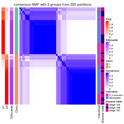
consensus_heatmap(res, k = 3)
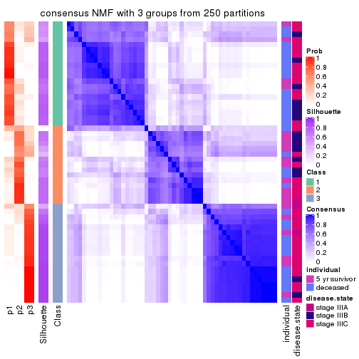
consensus_heatmap(res, k = 4)
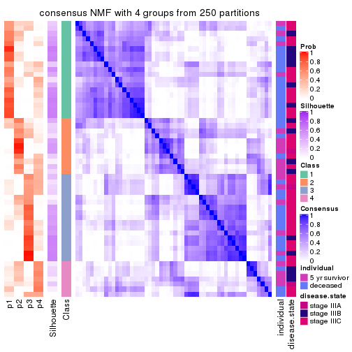
consensus_heatmap(res, k = 5)
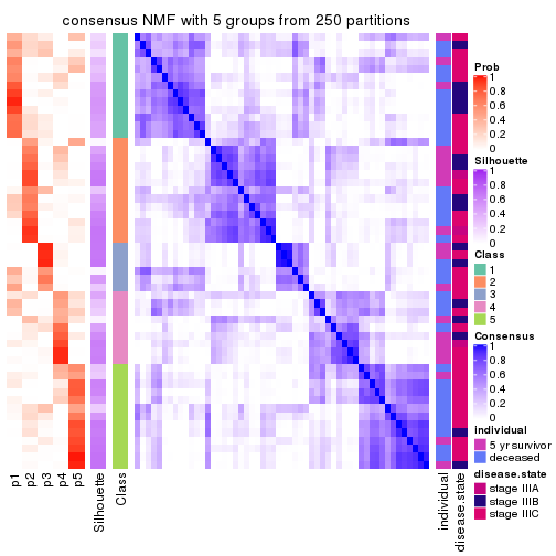
consensus_heatmap(res, k = 6)
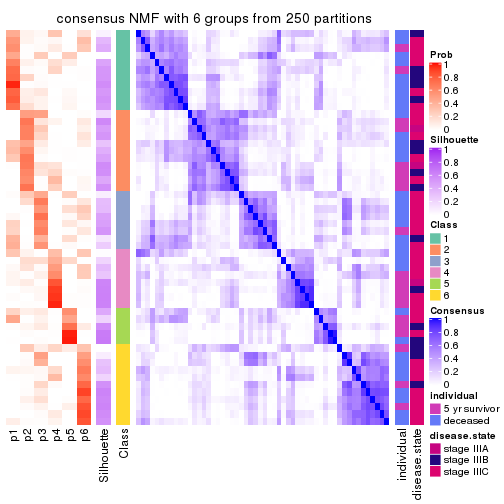
Heatmaps for the membership of samples in all partitions to see how consistent they are:
membership_heatmap(res, k = 2)
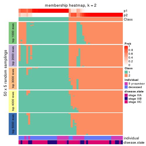
membership_heatmap(res, k = 3)
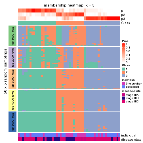
membership_heatmap(res, k = 4)
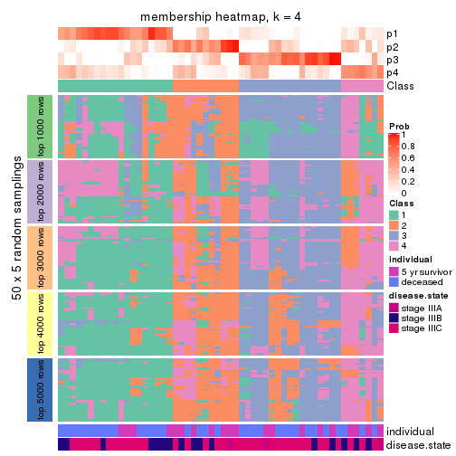
membership_heatmap(res, k = 5)
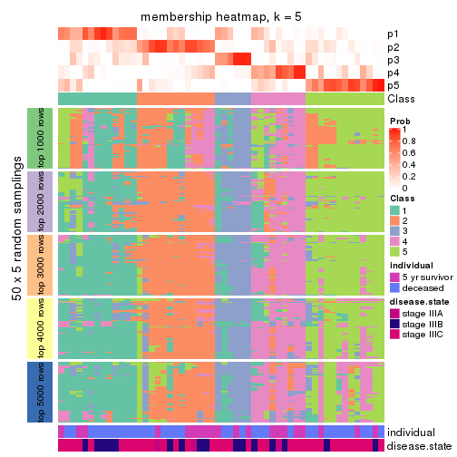
membership_heatmap(res, k = 6)
As soon as we have had the classes for columns, we can look for signatures which are significantly different between classes which can be candidate marks for certain classes. Following are the heatmaps for signatures.
Signature heatmaps where rows are scaled:
get_signatures(res, k = 2)
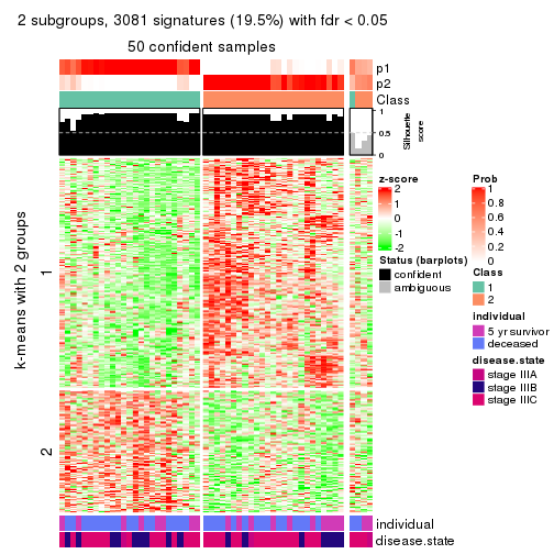
get_signatures(res, k = 3)
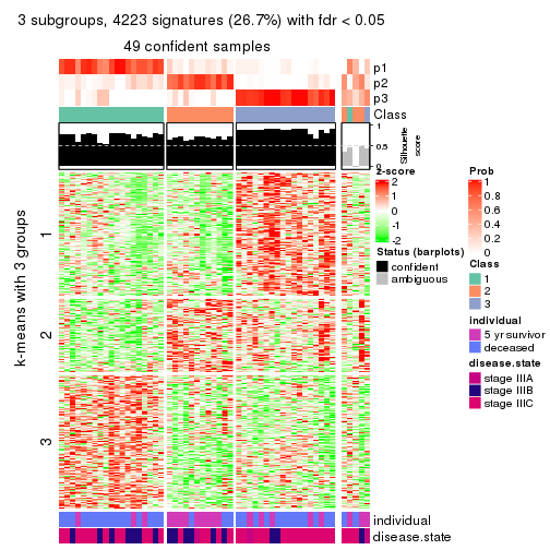
get_signatures(res, k = 4)
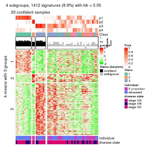
get_signatures(res, k = 5)
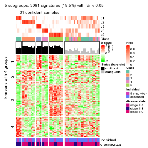
get_signatures(res, k = 6)
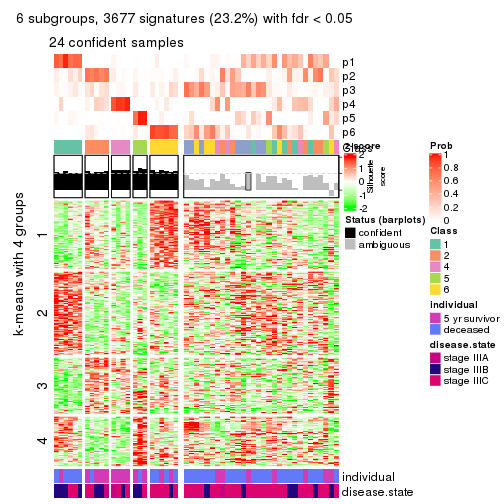
Signature heatmaps where rows are not scaled:
get_signatures(res, k = 2, scale_rows = FALSE)
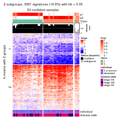
get_signatures(res, k = 3, scale_rows = FALSE)
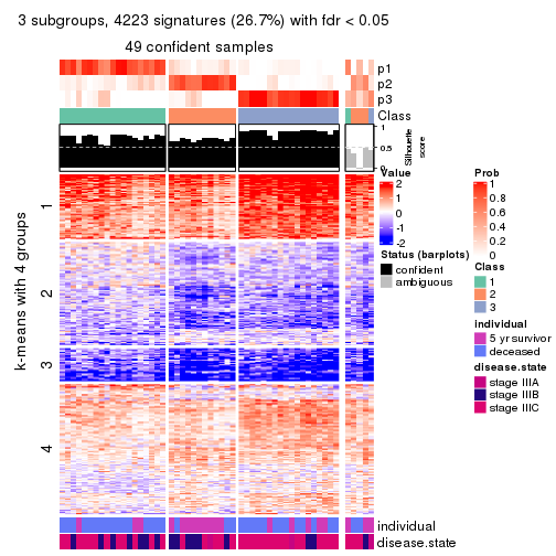
get_signatures(res, k = 4, scale_rows = FALSE)
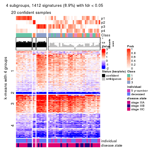
get_signatures(res, k = 5, scale_rows = FALSE)
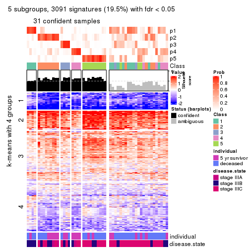
get_signatures(res, k = 6, scale_rows = FALSE)
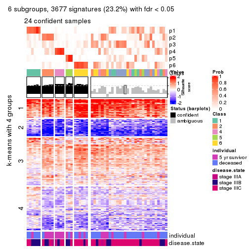
Compare the overlap of signatures from different k:
compare_signatures(res)
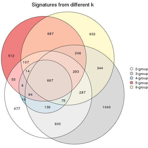
get_signature() returns a data frame invisibly. TO get the list of signatures, the function
call should be assigned to a variable explicitly. In following code, if plot argument is set
to FALSE, no heatmap is plotted while only the differential analysis is performed.
# code only for demonstration
tb = get_signature(res, k = ..., plot = FALSE)
An example of the output of tb is:
#>   which_row         fdr    mean_1    mean_2 scaled_mean_1 scaled_mean_2 km
#> 1        38 0.042760348  8.373488  9.131774    -0.5533452     0.5164555  1
#> 2        40 0.018707592  7.106213  8.469186    -0.6173731     0.5762149  1
#> 3        55 0.019134737 10.221463 11.207825    -0.6159697     0.5749050  1
#> 4        59 0.006059896  5.921854  7.869574    -0.6899429     0.6439467  1
#> 5        60 0.018055526  8.928898 10.211722    -0.6204761     0.5791110  1
#> 6        98 0.009384629 15.714769 14.887706     0.6635654    -0.6193277  2
...
The columns in tb are:
which_row: row indices corresponding to the input matrix.fdr: FDR for the differential test. mean_x: The mean value in group x.scaled_mean_x: The mean value in group x after rows are scaled.km: Row groups if k-means clustering is applied to rows.UMAP plot which shows how samples are separated.
dimension_reduction(res, k = 2, method = "UMAP")
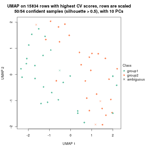
dimension_reduction(res, k = 3, method = "UMAP")
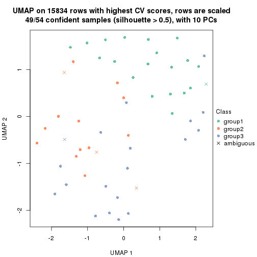
dimension_reduction(res, k = 4, method = "UMAP")
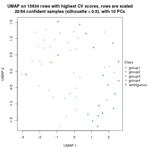
dimension_reduction(res, k = 5, method = "UMAP")
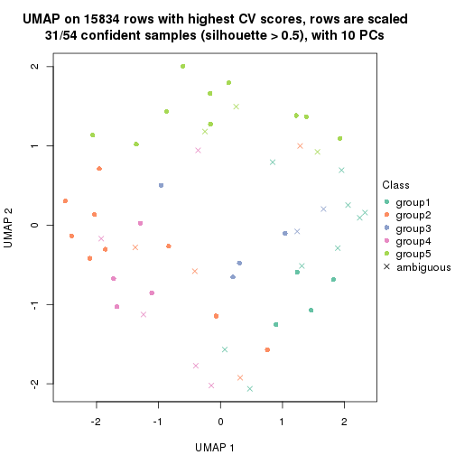
dimension_reduction(res, k = 6, method = "UMAP")
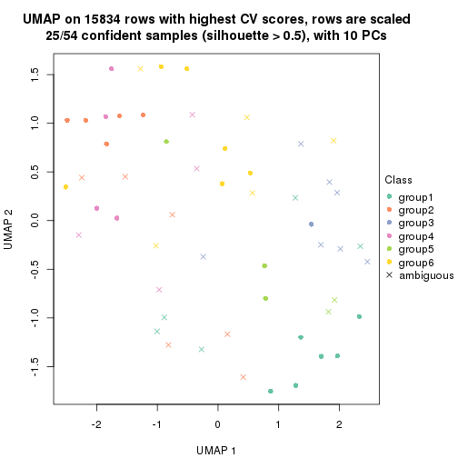
Following heatmap shows how subgroups are split when increasing k:
collect_classes(res)
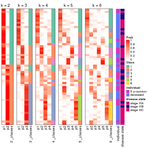
Test correlation between subgroups and known annotations. If the known annotation is numeric, one-way ANOVA test is applied, and if the known annotation is discrete, chi-squared contingency table test is applied.
test_to_known_factors(res)
#>         n individual(p) disease.state(p) k
#> CV:NMF 50        0.7683           0.8290 2
#> CV:NMF 49        0.0025           0.1214 3
#> CV:NMF 20        0.0231           0.0427 4
#> CV:NMF 31        0.0749           0.1093 5
#> CV:NMF 25        0.0683           0.5333 6
If matrix rows can be associated to genes, consider to use functional_enrichment(res,
...) to perform function enrichment for the signature genes. See this vignette for more detailed explanations.
The object with results only for a single top-value method and a single partition method can be extracted as:
res = res_list["MAD", "hclust"]
# you can also extract it by
# res = res_list["MAD:hclust"]
A summary of res and all the functions that can be applied to it:
res
#> A 'ConsensusPartition' object with k = 2, 3, 4, 5, 6.
#>   On a matrix with 15834 rows and 54 columns.
#>   Top rows (1000, 2000, 3000, 4000, 5000) are extracted by 'MAD' method.
#>   Subgroups are detected by 'hclust' method.
#>   Performed in total 1250 partitions by row resampling.
#>   Best k for subgroups seems to be 6.
#>
#> Following methods can be applied to this 'ConsensusPartition' object:
#>  [1] "cola_report"             "collect_classes"         "collect_plots"
#>  [4] "collect_stats"           "colnames"                "compare_signatures"
#>  [7] "consensus_heatmap"       "dimension_reduction"     "functional_enrichment"
#> [10] "get_anno_col"            "get_anno"                "get_classes"
#> [13] "get_consensus"           "get_matrix"              "get_membership"
#> [16] "get_param"               "get_signatures"          "get_stats"
#> [19] "is_best_k"               "is_stable_k"             "membership_heatmap"
#> [22] "ncol"                    "nrow"                    "plot_ecdf"
#> [25] "rownames"                "select_partition_number" "show"
#> [28] "suggest_best_k"          "test_to_known_factors"
collect_plots() function collects all the plots made from res for all k (number of partitions)
into one single page to provide an easy and fast comparison between different k.
collect_plots(res)
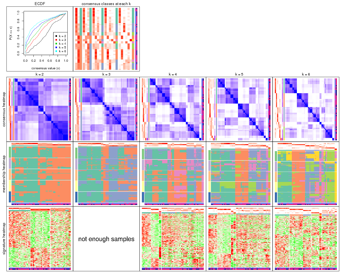
The plots are:
k and the heatmap of
predicted classes for each k.k.k.k.All the plots in panels can be made by individual functions and they are plotted later in this section.
select_partition_number() produces several plots showing different
statistics for choosing “optimized” k. There are following statistics:
k;k, the area increased is defined as \(A_k - A_{k-1}\).The detailed explanations of these statistics can be found in the cola vignette.
Generally speaking, lower PAC score, higher mean silhouette score or higher
concordance corresponds to better partition. Rand index and Jaccard index
measure how similar the current partition is compared to partition with k-1.
If they are too similar, we won't accept k is better than k-1.
select_partition_number(res)
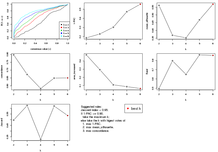
The numeric values for all these statistics can be obtained by get_stats().
get_stats(res)
#>   k 1-PAC mean_silhouette concordance area_increased  Rand Jaccard
#> 2 2 0.187           0.562       0.797         0.4742 0.497   0.497
#> 3 3 0.230           0.369       0.672         0.2941 0.795   0.624
#> 4 4 0.304           0.352       0.583         0.1091 0.649   0.329
#> 5 5 0.472           0.468       0.649         0.0871 0.860   0.620
#> 6 6 0.555           0.569       0.650         0.0641 0.854   0.537
suggest_best_k() suggests the best \(k\) based on these statistics. The rules are as follows:
suggest_best_k(res)
#> [1] 6
Following shows the table of the partitions (You need to click the show/hide
code output link to see it). The membership matrix (columns with name p*)
is inferred by
clue::cl_consensus()
function with the SE method. Basically the value in the membership matrix
represents the probability to belong to a certain group. The finall class
label for an item is determined with the group with highest probability it
belongs to.
In get_classes() function, the entropy is calculated from the membership
matrix and the silhouette score is calculated from the consensus matrix.
cbind(get_classes(res, k = 2), get_membership(res, k = 2))
#>           class entropy silhouette    p1    p2
#> GSM311939     2  0.3584      0.730 0.068 0.932
#> GSM311963     2  0.3584      0.730 0.068 0.932
#> GSM311973     2  0.6801      0.684 0.180 0.820
#> GSM311940     2  0.3584      0.730 0.068 0.932
#> GSM311953     2  0.4690      0.726 0.100 0.900
#> GSM311974     2  0.4690      0.726 0.100 0.900
#> GSM311975     1  0.9710      0.365 0.600 0.400
#> GSM311977     2  0.3584      0.730 0.068 0.932
#> GSM311982     1  0.1184      0.744 0.984 0.016
#> GSM311990     2  0.4690      0.720 0.100 0.900
#> GSM311943     1  0.8608      0.598 0.716 0.284
#> GSM311944     1  0.1184      0.744 0.984 0.016
#> GSM311946     2  0.4022      0.729 0.080 0.920
#> GSM311956     2  0.4939      0.724 0.108 0.892
#> GSM311967     2  0.2603      0.711 0.044 0.956
#> GSM311968     2  0.9732      0.424 0.404 0.596
#> GSM311972     1  0.2236      0.748 0.964 0.036
#> GSM311980     2  0.6801      0.684 0.180 0.820
#> GSM311981     2  0.9686      0.123 0.396 0.604
#> GSM311988     2  0.3584      0.730 0.068 0.932
#> GSM311957     1  0.9323      0.219 0.652 0.348
#> GSM311960     1  0.9944     -0.144 0.544 0.456
#> GSM311971     1  0.1184      0.741 0.984 0.016
#> GSM311976     1  0.5408      0.693 0.876 0.124
#> GSM311978     1  0.1184      0.741 0.984 0.016
#> GSM311979     1  0.1184      0.741 0.984 0.016
#> GSM311983     1  0.7299      0.668 0.796 0.204
#> GSM311986     2  0.9522      0.375 0.372 0.628
#> GSM311991     2  0.9775      0.080 0.412 0.588
#> GSM311938     2  0.9000      0.477 0.316 0.684
#> GSM311941     2  0.9963      0.215 0.464 0.536
#> GSM311942     2  0.9993      0.246 0.484 0.516
#> GSM311945     2  1.0000      0.213 0.496 0.504
#> GSM311947     2  0.2948      0.712 0.052 0.948
#> GSM311948     2  0.5294      0.721 0.120 0.880
#> GSM311949     1  0.5408      0.693 0.876 0.124
#> GSM311950     2  0.0672      0.699 0.008 0.992
#> GSM311951     2  0.9993      0.246 0.484 0.516
#> GSM311952     1  0.8608      0.598 0.716 0.284
#> GSM311954     2  0.9286      0.427 0.344 0.656
#> GSM311955     1  0.9608      0.418 0.616 0.384
#> GSM311958     1  0.4815      0.740 0.896 0.104
#> GSM311959     2  0.9286      0.427 0.344 0.656
#> GSM311961     1  0.7139      0.673 0.804 0.196
#> GSM311962     1  0.3274      0.749 0.940 0.060
#> GSM311964     1  0.5408      0.693 0.876 0.124
#> GSM311965     2  0.9732      0.424 0.404 0.596
#> GSM311966     1  0.3114      0.748 0.944 0.056
#> GSM311969     1  0.8608      0.598 0.716 0.284
#> GSM311970     2  0.0672      0.699 0.008 0.992
#> GSM311984     1  0.7299      0.668 0.796 0.204
#> GSM311985     1  0.2043      0.747 0.968 0.032
#> GSM311987     2  0.9286      0.427 0.344 0.656
#> GSM311989     1  0.9944     -0.144 0.544 0.456
cbind(get_classes(res, k = 3), get_membership(res, k = 3))
#>           class entropy silhouette    p1    p2    p3
#> GSM311939     2   0.630     0.1739 0.000 0.520 0.480
#> GSM311963     2   0.630     0.1739 0.000 0.520 0.480
#> GSM311973     3   0.761     0.1625 0.064 0.316 0.620
#> GSM311940     3   0.631    -0.2417 0.000 0.492 0.508
#> GSM311953     3   0.583     0.0924 0.000 0.340 0.660
#> GSM311974     3   0.581     0.1003 0.000 0.336 0.664
#> GSM311975     1   0.770     0.4737 0.664 0.232 0.104
#> GSM311977     3   0.631    -0.2417 0.000 0.492 0.508
#> GSM311982     1   0.506     0.6918 0.756 0.000 0.244
#> GSM311990     3   0.659     0.2940 0.060 0.208 0.732
#> GSM311943     1   0.635     0.6098 0.768 0.092 0.140
#> GSM311944     1   0.506     0.6918 0.756 0.000 0.244
#> GSM311946     3   0.662     0.0428 0.012 0.388 0.600
#> GSM311956     3   0.571     0.1256 0.000 0.320 0.680
#> GSM311967     3   0.708     0.1463 0.032 0.356 0.612
#> GSM311968     3   0.441     0.4245 0.160 0.008 0.832
#> GSM311972     1   0.277     0.7476 0.916 0.004 0.080
#> GSM311980     3   0.759     0.1690 0.064 0.312 0.624
#> GSM311981     2   0.790    -0.1187 0.440 0.504 0.056
#> GSM311988     2   0.630     0.1739 0.000 0.520 0.480
#> GSM311957     3   0.614     0.0164 0.404 0.000 0.596
#> GSM311960     3   0.536     0.3139 0.276 0.000 0.724
#> GSM311971     1   0.497     0.6946 0.764 0.000 0.236
#> GSM311976     1   0.571     0.5988 0.680 0.000 0.320
#> GSM311978     1   0.489     0.6996 0.772 0.000 0.228
#> GSM311979     1   0.497     0.6946 0.764 0.000 0.236
#> GSM311983     1   0.341     0.6739 0.876 0.124 0.000
#> GSM311986     3   0.866     0.2379 0.408 0.104 0.488
#> GSM311991     2   0.792    -0.1559 0.456 0.488 0.056
#> GSM311938     3   0.971     0.1769 0.352 0.224 0.424
#> GSM311941     3   0.700     0.2150 0.428 0.020 0.552
#> GSM311942     3   0.493     0.3945 0.232 0.000 0.768
#> GSM311945     3   0.506     0.3797 0.244 0.000 0.756
#> GSM311947     3   0.695     0.1680 0.032 0.332 0.636
#> GSM311948     3   0.497     0.2869 0.012 0.188 0.800
#> GSM311949     1   0.571     0.5988 0.680 0.000 0.320
#> GSM311950     2   0.375     0.3730 0.000 0.856 0.144
#> GSM311951     3   0.493     0.3945 0.232 0.000 0.768
#> GSM311952     1   0.635     0.6098 0.768 0.092 0.140
#> GSM311954     3   0.892     0.2440 0.380 0.128 0.492
#> GSM311955     1   0.803     0.4706 0.656 0.164 0.180
#> GSM311958     1   0.280     0.7365 0.924 0.016 0.060
#> GSM311959     3   0.892     0.2440 0.380 0.128 0.492
#> GSM311961     1   0.500     0.6925 0.832 0.124 0.044
#> GSM311962     1   0.217     0.7471 0.944 0.008 0.048
#> GSM311964     1   0.571     0.5988 0.680 0.000 0.320
#> GSM311965     3   0.441     0.4245 0.160 0.008 0.832
#> GSM311966     1   0.210     0.7474 0.944 0.004 0.052
#> GSM311969     1   0.635     0.6098 0.768 0.092 0.140
#> GSM311970     2   0.375     0.3730 0.000 0.856 0.144
#> GSM311984     1   0.341     0.6739 0.876 0.124 0.000
#> GSM311985     1   0.268     0.7475 0.920 0.004 0.076
#> GSM311987     3   0.892     0.2440 0.380 0.128 0.492
#> GSM311989     3   0.536     0.3139 0.276 0.000 0.724
cbind(get_classes(res, k = 4), get_membership(res, k = 4))
#>           class entropy silhouette    p1    p2    p3    p4
#> GSM311939     2  0.3726     0.3981 0.000 0.788 0.000 0.212
#> GSM311963     2  0.3726     0.3981 0.000 0.788 0.000 0.212
#> GSM311973     2  0.3573     0.5453 0.100 0.864 0.028 0.008
#> GSM311940     2  0.3356     0.4514 0.000 0.824 0.000 0.176
#> GSM311953     2  0.1174     0.5772 0.020 0.968 0.000 0.012
#> GSM311974     2  0.1362     0.5789 0.020 0.964 0.004 0.012
#> GSM311975     1  0.8404    -0.2800 0.416 0.052 0.388 0.144
#> GSM311977     2  0.3356     0.4514 0.000 0.824 0.000 0.176
#> GSM311982     1  0.1042     0.5456 0.972 0.020 0.008 0.000
#> GSM311990     2  0.8308     0.2770 0.024 0.440 0.304 0.232
#> GSM311943     3  0.7081     0.3366 0.424 0.124 0.452 0.000
#> GSM311944     1  0.1042     0.5456 0.972 0.020 0.008 0.000
#> GSM311946     2  0.3138     0.5624 0.024 0.896 0.020 0.060
#> GSM311956     2  0.1297     0.5812 0.020 0.964 0.016 0.000
#> GSM311967     2  0.7830     0.1828 0.000 0.400 0.268 0.332
#> GSM311968     2  0.8574    -0.0185 0.336 0.364 0.272 0.028
#> GSM311972     1  0.3306     0.4157 0.840 0.000 0.156 0.004
#> GSM311980     2  0.3670     0.5461 0.100 0.860 0.032 0.008
#> GSM311981     3  0.5771    -0.2419 0.000 0.028 0.512 0.460
#> GSM311988     2  0.3726     0.3981 0.000 0.788 0.000 0.212
#> GSM311957     1  0.6854     0.3673 0.600 0.204 0.196 0.000
#> GSM311960     1  0.8200     0.2422 0.488 0.236 0.248 0.028
#> GSM311971     1  0.0469     0.5448 0.988 0.012 0.000 0.000
#> GSM311976     1  0.3972     0.5304 0.840 0.080 0.080 0.000
#> GSM311978     1  0.0804     0.5422 0.980 0.012 0.008 0.000
#> GSM311979     1  0.0469     0.5448 0.988 0.012 0.000 0.000
#> GSM311983     3  0.5158     0.1855 0.472 0.000 0.524 0.004
#> GSM311986     3  0.8576     0.4080 0.140 0.312 0.472 0.076
#> GSM311991     3  0.5755    -0.2117 0.000 0.028 0.528 0.444
#> GSM311938     3  0.8590     0.3189 0.096 0.368 0.432 0.104
#> GSM311941     3  0.7717     0.2764 0.264 0.288 0.448 0.000
#> GSM311942     1  0.8487     0.1369 0.416 0.284 0.272 0.028
#> GSM311945     1  0.8438     0.1645 0.432 0.272 0.268 0.028
#> GSM311947     2  0.7806     0.2107 0.000 0.412 0.264 0.324
#> GSM311948     2  0.3907     0.5452 0.032 0.828 0.140 0.000
#> GSM311949     1  0.3972     0.5304 0.840 0.080 0.080 0.000
#> GSM311950     4  0.3266     1.0000 0.000 0.168 0.000 0.832
#> GSM311951     1  0.8487     0.1369 0.416 0.284 0.272 0.028
#> GSM311952     3  0.7081     0.3366 0.424 0.124 0.452 0.000
#> GSM311954     3  0.8139     0.4061 0.100 0.320 0.508 0.072
#> GSM311955     3  0.8438     0.3828 0.360 0.152 0.436 0.052
#> GSM311958     1  0.5188     0.2298 0.704 0.016 0.268 0.012
#> GSM311959     3  0.8139     0.4061 0.100 0.320 0.508 0.072
#> GSM311961     1  0.5334    -0.2178 0.508 0.004 0.484 0.004
#> GSM311962     1  0.4122     0.3197 0.760 0.004 0.236 0.000
#> GSM311964     1  0.3972     0.5304 0.840 0.080 0.080 0.000
#> GSM311965     2  0.8574    -0.0185 0.336 0.364 0.272 0.028
#> GSM311966     1  0.4053     0.3291 0.768 0.004 0.228 0.000
#> GSM311969     3  0.7081     0.3366 0.424 0.124 0.452 0.000
#> GSM311970     4  0.3266     1.0000 0.000 0.168 0.000 0.832
#> GSM311984     3  0.5158     0.1855 0.472 0.000 0.524 0.004
#> GSM311985     1  0.3123     0.4177 0.844 0.000 0.156 0.000
#> GSM311987     3  0.8139     0.4061 0.100 0.320 0.508 0.072
#> GSM311989     1  0.8200     0.2422 0.488 0.236 0.248 0.028
cbind(get_classes(res, k = 5), get_membership(res, k = 5))
#>           class entropy silhouette    p1    p2    p3    p4    p5
#> GSM311939     2  0.3551     0.6706 0.000 0.772 0.008 0.000 0.220
#> GSM311963     2  0.3551     0.6706 0.000 0.772 0.008 0.000 0.220
#> GSM311973     2  0.4133     0.6380 0.060 0.836 0.044 0.036 0.024
#> GSM311940     2  0.3246     0.7070 0.000 0.808 0.008 0.000 0.184
#> GSM311953     2  0.0162     0.7597 0.000 0.996 0.004 0.000 0.000
#> GSM311974     2  0.0324     0.7596 0.000 0.992 0.004 0.000 0.004
#> GSM311975     3  0.7460     0.2740 0.380 0.008 0.388 0.192 0.032
#> GSM311977     2  0.3246     0.7070 0.000 0.808 0.008 0.000 0.184
#> GSM311982     1  0.1518     0.5295 0.952 0.012 0.016 0.000 0.020
#> GSM311990     3  0.7729     0.0165 0.000 0.176 0.492 0.200 0.132
#> GSM311943     3  0.6587     0.3806 0.344 0.016 0.496 0.144 0.000
#> GSM311944     1  0.1518     0.5295 0.952 0.012 0.016 0.000 0.020
#> GSM311946     2  0.2300     0.7200 0.000 0.904 0.072 0.000 0.024
#> GSM311956     2  0.0703     0.7512 0.000 0.976 0.000 0.000 0.024
#> GSM311967     3  0.7656    -0.0567 0.000 0.148 0.508 0.168 0.176
#> GSM311968     1  0.9601     0.2824 0.292 0.232 0.200 0.084 0.192
#> GSM311972     1  0.3242     0.3868 0.816 0.000 0.172 0.012 0.000
#> GSM311980     2  0.4219     0.6350 0.060 0.832 0.044 0.036 0.028
#> GSM311981     4  0.3456     0.9692 0.000 0.000 0.184 0.800 0.016
#> GSM311988     2  0.3551     0.6706 0.000 0.772 0.008 0.000 0.220
#> GSM311957     1  0.8185     0.4459 0.536 0.136 0.116 0.068 0.144
#> GSM311960     1  0.8807     0.4194 0.460 0.124 0.144 0.084 0.188
#> GSM311971     1  0.0000     0.5249 1.000 0.000 0.000 0.000 0.000
#> GSM311976     1  0.5044     0.5213 0.772 0.072 0.084 0.064 0.008
#> GSM311978     1  0.0290     0.5215 0.992 0.000 0.008 0.000 0.000
#> GSM311979     1  0.0000     0.5249 1.000 0.000 0.000 0.000 0.000
#> GSM311983     3  0.6693     0.2701 0.392 0.000 0.404 0.200 0.004
#> GSM311986     3  0.5269     0.4194 0.072 0.080 0.768 0.052 0.028
#> GSM311991     4  0.3109     0.9695 0.000 0.000 0.200 0.800 0.000
#> GSM311938     3  0.5471     0.3369 0.036 0.196 0.712 0.024 0.032
#> GSM311941     3  0.6926     0.3412 0.216 0.076 0.608 0.024 0.076
#> GSM311942     1  0.9192     0.3688 0.388 0.124 0.216 0.084 0.188
#> GSM311945     1  0.9128     0.3804 0.404 0.124 0.200 0.084 0.188
#> GSM311947     3  0.7593    -0.0337 0.000 0.152 0.516 0.148 0.184
#> GSM311948     2  0.2997     0.6256 0.000 0.840 0.012 0.000 0.148
#> GSM311949     1  0.5044     0.5213 0.772 0.072 0.084 0.064 0.008
#> GSM311950     5  0.3577     1.0000 0.000 0.160 0.000 0.032 0.808
#> GSM311951     1  0.9192     0.3688 0.388 0.124 0.216 0.084 0.188
#> GSM311952     3  0.6587     0.3806 0.344 0.016 0.496 0.144 0.000
#> GSM311954     3  0.3361     0.4083 0.036 0.080 0.860 0.024 0.000
#> GSM311955     3  0.5266     0.4217 0.292 0.020 0.648 0.040 0.000
#> GSM311958     1  0.4288     0.1894 0.664 0.000 0.324 0.012 0.000
#> GSM311959     3  0.3361     0.4083 0.036 0.080 0.860 0.024 0.000
#> GSM311961     1  0.6744    -0.2977 0.436 0.004 0.372 0.184 0.004
#> GSM311962     1  0.3861     0.2864 0.728 0.000 0.264 0.008 0.000
#> GSM311964     1  0.5044     0.5213 0.772 0.072 0.084 0.064 0.008
#> GSM311965     1  0.9601     0.2824 0.292 0.232 0.200 0.084 0.192
#> GSM311966     1  0.3961     0.2967 0.736 0.000 0.248 0.016 0.000
#> GSM311969     3  0.6587     0.3806 0.344 0.016 0.496 0.144 0.000
#> GSM311970     5  0.3577     1.0000 0.000 0.160 0.000 0.032 0.808
#> GSM311984     3  0.6693     0.2701 0.392 0.000 0.404 0.200 0.004
#> GSM311985     1  0.3132     0.3869 0.820 0.000 0.172 0.008 0.000
#> GSM311987     3  0.3361     0.4083 0.036 0.080 0.860 0.024 0.000
#> GSM311989     1  0.8807     0.4194 0.460 0.124 0.144 0.084 0.188
cbind(get_classes(res, k = 6), get_membership(res, k = 6))
#>           class entropy silhouette    p1    p2    p3    p4    p5    p6
#> GSM311939     2  0.2214      0.730 0.000 0.888 0.016 0.096 0.000 0.000
#> GSM311963     2  0.2214      0.730 0.000 0.888 0.016 0.096 0.000 0.000
#> GSM311973     2  0.4339      0.655 0.060 0.684 0.000 0.000 0.256 0.000
#> GSM311940     2  0.2237      0.761 0.000 0.896 0.004 0.080 0.020 0.000
#> GSM311953     2  0.2135      0.788 0.000 0.872 0.000 0.000 0.128 0.000
#> GSM311974     2  0.2178      0.788 0.000 0.868 0.000 0.000 0.132 0.000
#> GSM311975     3  0.7105      0.400 0.220 0.000 0.528 0.040 0.092 0.120
#> GSM311977     2  0.2237      0.761 0.000 0.896 0.004 0.080 0.020 0.000
#> GSM311982     1  0.3104      0.646 0.800 0.000 0.016 0.000 0.184 0.000
#> GSM311990     5  0.5704     -0.200 0.000 0.020 0.008 0.264 0.596 0.112
#> GSM311943     3  0.3468      0.616 0.092 0.004 0.816 0.000 0.088 0.000
#> GSM311944     1  0.3104      0.646 0.800 0.000 0.016 0.000 0.184 0.000
#> GSM311946     2  0.3532      0.753 0.000 0.816 0.012 0.024 0.136 0.012
#> GSM311956     2  0.2416      0.780 0.000 0.844 0.000 0.000 0.156 0.000
#> GSM311967     4  0.7451      0.179 0.000 0.028 0.068 0.384 0.324 0.196
#> GSM311968     5  0.3894      0.661 0.152 0.064 0.008 0.000 0.776 0.000
#> GSM311972     1  0.2812      0.713 0.856 0.000 0.096 0.000 0.000 0.048
#> GSM311980     2  0.4360      0.652 0.060 0.680 0.000 0.000 0.260 0.000
#> GSM311981     6  0.0458      0.968 0.000 0.000 0.000 0.016 0.000 0.984
#> GSM311988     2  0.2214      0.730 0.000 0.888 0.016 0.096 0.000 0.000
#> GSM311957     5  0.5642      0.321 0.428 0.024 0.068 0.000 0.476 0.004
#> GSM311960     5  0.3615      0.617 0.292 0.008 0.000 0.000 0.700 0.000
#> GSM311971     1  0.1285      0.719 0.944 0.000 0.000 0.000 0.052 0.004
#> GSM311976     1  0.4387      0.565 0.748 0.020 0.060 0.000 0.168 0.004
#> GSM311978     1  0.1333      0.721 0.944 0.000 0.000 0.000 0.048 0.008
#> GSM311979     1  0.1285      0.719 0.944 0.000 0.000 0.000 0.052 0.004
#> GSM311983     3  0.1757      0.537 0.076 0.000 0.916 0.000 0.008 0.000
#> GSM311986     3  0.6501      0.418 0.000 0.004 0.488 0.224 0.252 0.032
#> GSM311991     6  0.0146      0.968 0.004 0.000 0.000 0.000 0.000 0.996
#> GSM311938     3  0.9189      0.304 0.048 0.180 0.336 0.152 0.188 0.096
#> GSM311941     5  0.8164     -0.283 0.244 0.004 0.252 0.128 0.336 0.036
#> GSM311942     5  0.3190      0.684 0.220 0.000 0.008 0.000 0.772 0.000
#> GSM311945     5  0.3329      0.679 0.236 0.004 0.004 0.000 0.756 0.000
#> GSM311947     4  0.7319      0.194 0.000 0.028 0.068 0.384 0.360 0.160
#> GSM311948     2  0.3371      0.663 0.000 0.708 0.000 0.000 0.292 0.000
#> GSM311949     1  0.4387      0.565 0.748 0.020 0.060 0.000 0.168 0.004
#> GSM311950     4  0.3309      0.246 0.000 0.280 0.000 0.720 0.000 0.000
#> GSM311951     5  0.3190      0.684 0.220 0.000 0.008 0.000 0.772 0.000
#> GSM311952     3  0.3468      0.616 0.092 0.004 0.816 0.000 0.088 0.000
#> GSM311954     3  0.8204      0.393 0.056 0.004 0.356 0.220 0.260 0.104
#> GSM311955     3  0.6544      0.574 0.144 0.004 0.608 0.024 0.136 0.084
#> GSM311958     1  0.4949      0.534 0.672 0.000 0.248 0.008 0.024 0.048
#> GSM311959     3  0.8204      0.393 0.056 0.004 0.356 0.220 0.260 0.104
#> GSM311961     3  0.2734      0.508 0.116 0.004 0.860 0.000 0.016 0.004
#> GSM311962     1  0.3789      0.649 0.760 0.000 0.196 0.000 0.004 0.040
#> GSM311964     1  0.4420      0.563 0.744 0.020 0.060 0.000 0.172 0.004
#> GSM311965     5  0.3894      0.661 0.152 0.064 0.008 0.000 0.776 0.000
#> GSM311966     1  0.3695      0.661 0.772 0.000 0.184 0.000 0.004 0.040
#> GSM311969     3  0.3516      0.615 0.096 0.004 0.812 0.000 0.088 0.000
#> GSM311970     4  0.3309      0.246 0.000 0.280 0.000 0.720 0.000 0.000
#> GSM311984     3  0.1757      0.537 0.076 0.000 0.916 0.000 0.008 0.000
#> GSM311985     1  0.2747      0.714 0.860 0.000 0.096 0.000 0.000 0.044
#> GSM311987     3  0.8204      0.393 0.056 0.004 0.356 0.220 0.260 0.104
#> GSM311989     5  0.3615      0.617 0.292 0.008 0.000 0.000 0.700 0.000
Heatmaps for the consensus matrix. It visualizes the probability of two samples to be in a same group.
consensus_heatmap(res, k = 2)
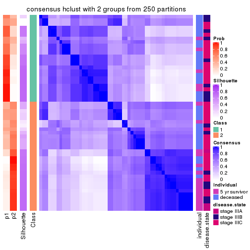
consensus_heatmap(res, k = 3)
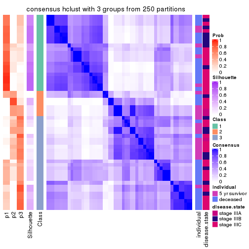
consensus_heatmap(res, k = 4)
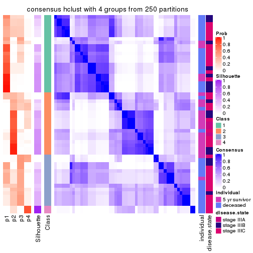
consensus_heatmap(res, k = 5)
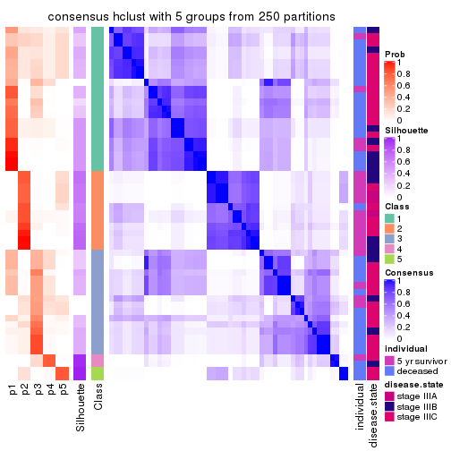
consensus_heatmap(res, k = 6)
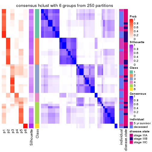
Heatmaps for the membership of samples in all partitions to see how consistent they are:
membership_heatmap(res, k = 2)
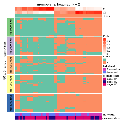
membership_heatmap(res, k = 3)
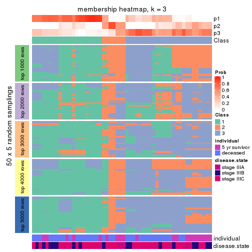
membership_heatmap(res, k = 4)
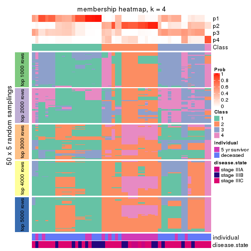
membership_heatmap(res, k = 5)
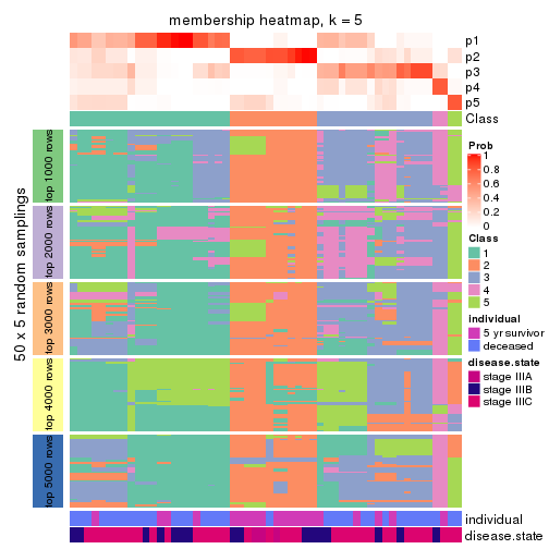
membership_heatmap(res, k = 6)
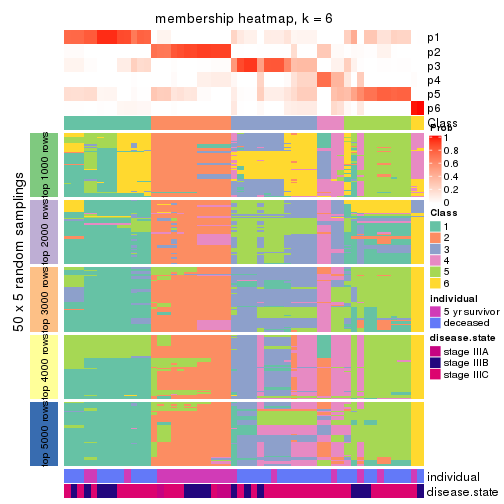
As soon as we have had the classes for columns, we can look for signatures which are significantly different between classes which can be candidate marks for certain classes. Following are the heatmaps for signatures.
Signature heatmaps where rows are scaled:
get_signatures(res, k = 2)
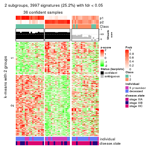
get_signatures(res, k = 3)

get_signatures(res, k = 4)
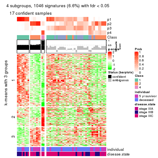
get_signatures(res, k = 5)
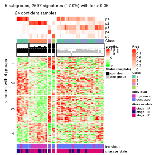
get_signatures(res, k = 6)
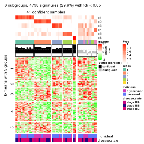
Signature heatmaps where rows are not scaled:
get_signatures(res, k = 2, scale_rows = FALSE)
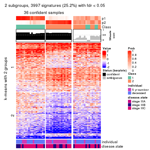
get_signatures(res, k = 3, scale_rows = FALSE)

get_signatures(res, k = 4, scale_rows = FALSE)
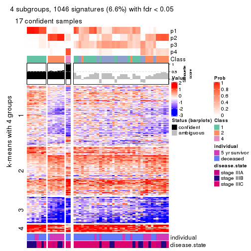
get_signatures(res, k = 5, scale_rows = FALSE)
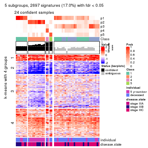
get_signatures(res, k = 6, scale_rows = FALSE)
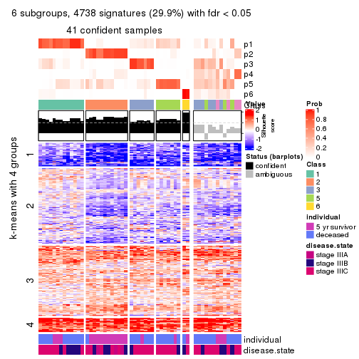
Compare the overlap of signatures from different k:
compare_signatures(res)
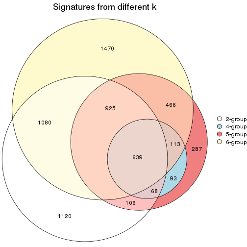
get_signature() returns a data frame invisibly. TO get the list of signatures, the function
call should be assigned to a variable explicitly. In following code, if plot argument is set
to FALSE, no heatmap is plotted while only the differential analysis is performed.
# code only for demonstration
tb = get_signature(res, k = ..., plot = FALSE)
An example of the output of tb is:
#>   which_row         fdr    mean_1    mean_2 scaled_mean_1 scaled_mean_2 km
#> 1        38 0.042760348  8.373488  9.131774    -0.5533452     0.5164555  1
#> 2        40 0.018707592  7.106213  8.469186    -0.6173731     0.5762149  1
#> 3        55 0.019134737 10.221463 11.207825    -0.6159697     0.5749050  1
#> 4        59 0.006059896  5.921854  7.869574    -0.6899429     0.6439467  1
#> 5        60 0.018055526  8.928898 10.211722    -0.6204761     0.5791110  1
#> 6        98 0.009384629 15.714769 14.887706     0.6635654    -0.6193277  2
...
The columns in tb are:
which_row: row indices corresponding to the input matrix.fdr: FDR for the differential test. mean_x: The mean value in group x.scaled_mean_x: The mean value in group x after rows are scaled.km: Row groups if k-means clustering is applied to rows.UMAP plot which shows how samples are separated.
dimension_reduction(res, k = 2, method = "UMAP")
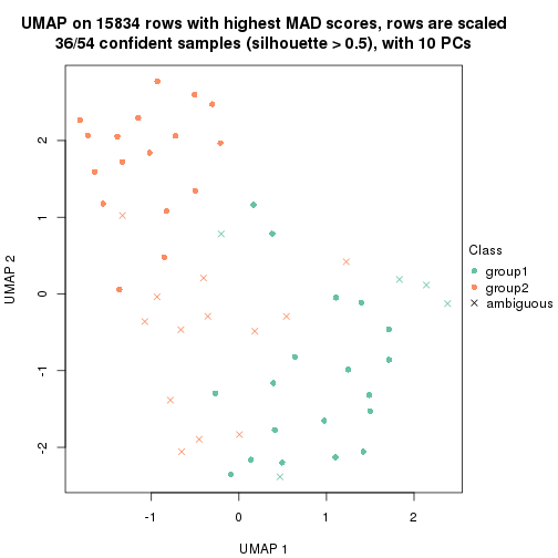
dimension_reduction(res, k = 3, method = "UMAP")
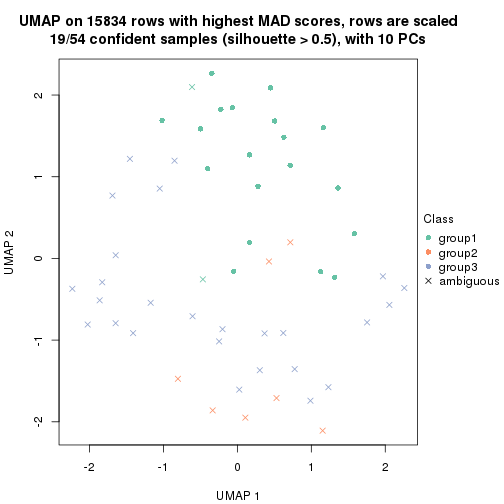
dimension_reduction(res, k = 4, method = "UMAP")
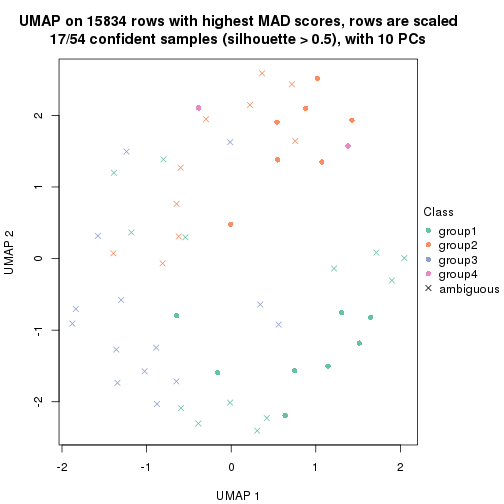
dimension_reduction(res, k = 5, method = "UMAP")
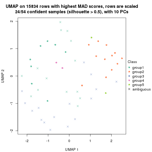
dimension_reduction(res, k = 6, method = "UMAP")
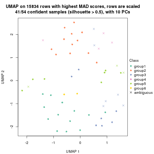
Following heatmap shows how subgroups are split when increasing k:
collect_classes(res)
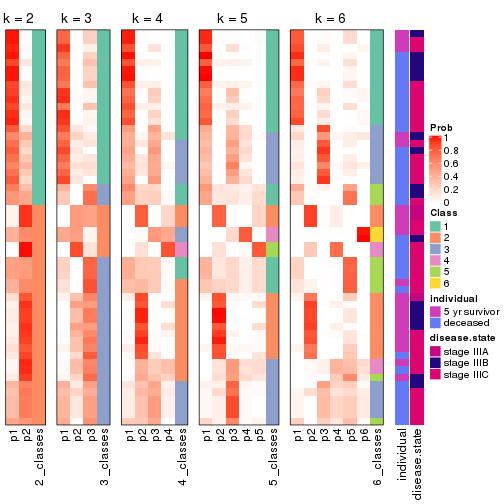
Test correlation between subgroups and known annotations. If the known annotation is numeric, one-way ANOVA test is applied, and if the known annotation is discrete, chi-squared contingency table test is applied.
test_to_known_factors(res)
#>             n individual(p) disease.state(p) k
#> MAD:hclust 36      0.002783            0.156 2
#> MAD:hclust 19            NA               NA 3
#> MAD:hclust 17      0.023067            0.328 4
#> MAD:hclust 24      0.007383            0.385 5
#> MAD:hclust 41      0.000945            0.195 6
If matrix rows can be associated to genes, consider to use functional_enrichment(res,
...) to perform function enrichment for the signature genes. See this vignette for more detailed explanations.
The object with results only for a single top-value method and a single partition method can be extracted as:
res = res_list["MAD", "kmeans"]
# you can also extract it by
# res = res_list["MAD:kmeans"]
A summary of res and all the functions that can be applied to it:
res
#> A 'ConsensusPartition' object with k = 2, 3, 4, 5, 6.
#>   On a matrix with 15834 rows and 54 columns.
#>   Top rows (1000, 2000, 3000, 4000, 5000) are extracted by 'MAD' method.
#>   Subgroups are detected by 'kmeans' method.
#>   Performed in total 1250 partitions by row resampling.
#>   Best k for subgroups seems to be 2.
#>
#> Following methods can be applied to this 'ConsensusPartition' object:
#>  [1] "cola_report"             "collect_classes"         "collect_plots"
#>  [4] "collect_stats"           "colnames"                "compare_signatures"
#>  [7] "consensus_heatmap"       "dimension_reduction"     "functional_enrichment"
#> [10] "get_anno_col"            "get_anno"                "get_classes"
#> [13] "get_consensus"           "get_matrix"              "get_membership"
#> [16] "get_param"               "get_signatures"          "get_stats"
#> [19] "is_best_k"               "is_stable_k"             "membership_heatmap"
#> [22] "ncol"                    "nrow"                    "plot_ecdf"
#> [25] "rownames"                "select_partition_number" "show"
#> [28] "suggest_best_k"          "test_to_known_factors"
collect_plots() function collects all the plots made from res for all k (number of partitions)
into one single page to provide an easy and fast comparison between different k.
collect_plots(res)
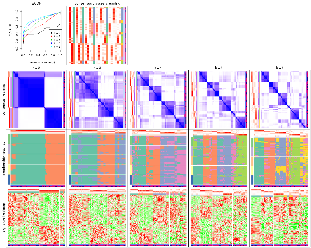
The plots are:
k and the heatmap of
predicted classes for each k.k.k.k.All the plots in panels can be made by individual functions and they are plotted later in this section.
select_partition_number() produces several plots showing different
statistics for choosing “optimized” k. There are following statistics:
k;k, the area increased is defined as \(A_k - A_{k-1}\).The detailed explanations of these statistics can be found in the cola vignette.
Generally speaking, lower PAC score, higher mean silhouette score or higher
concordance corresponds to better partition. Rand index and Jaccard index
measure how similar the current partition is compared to partition with k-1.
If they are too similar, we won't accept k is better than k-1.
select_partition_number(res)
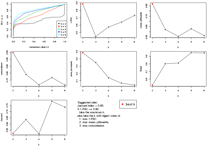
The numeric values for all these statistics can be obtained by get_stats().
get_stats(res)
#>   k 1-PAC mean_silhouette concordance area_increased  Rand Jaccard
#> 2 2 0.884           0.867       0.948         0.4842 0.525   0.525
#> 3 3 0.449           0.623       0.791         0.3503 0.802   0.635
#> 4 4 0.576           0.557       0.716         0.1407 0.812   0.521
#> 5 5 0.642           0.629       0.768         0.0675 0.946   0.782
#> 6 6 0.731           0.564       0.715         0.0418 0.943   0.736
suggest_best_k() suggests the best \(k\) based on these statistics. The rules are as follows:
suggest_best_k(res)
#> [1] 2
Following shows the table of the partitions (You need to click the show/hide
code output link to see it). The membership matrix (columns with name p*)
is inferred by
clue::cl_consensus()
function with the SE method. Basically the value in the membership matrix
represents the probability to belong to a certain group. The finall class
label for an item is determined with the group with highest probability it
belongs to.
In get_classes() function, the entropy is calculated from the membership
matrix and the silhouette score is calculated from the consensus matrix.
cbind(get_classes(res, k = 2), get_membership(res, k = 2))
#>           class entropy silhouette    p1    p2
#> GSM311939     2  0.0672      0.964 0.008 0.992
#> GSM311963     2  0.0672      0.964 0.008 0.992
#> GSM311973     2  0.0000      0.962 0.000 1.000
#> GSM311940     2  0.0672      0.964 0.008 0.992
#> GSM311953     2  0.0376      0.963 0.004 0.996
#> GSM311974     2  0.0000      0.962 0.000 1.000
#> GSM311975     1  0.0000      0.930 1.000 0.000
#> GSM311977     2  0.0672      0.964 0.008 0.992
#> GSM311982     1  0.0672      0.927 0.992 0.008
#> GSM311990     2  0.0376      0.964 0.004 0.996
#> GSM311943     1  0.0000      0.930 1.000 0.000
#> GSM311944     1  0.0672      0.927 0.992 0.008
#> GSM311946     2  0.0376      0.963 0.004 0.996
#> GSM311956     2  0.0000      0.962 0.000 1.000
#> GSM311967     2  0.0938      0.961 0.012 0.988
#> GSM311968     2  0.2603      0.923 0.044 0.956
#> GSM311972     1  0.0376      0.929 0.996 0.004
#> GSM311980     2  0.0000      0.962 0.000 1.000
#> GSM311981     1  0.0000      0.930 1.000 0.000
#> GSM311988     2  0.0672      0.964 0.008 0.992
#> GSM311957     1  0.0938      0.925 0.988 0.012
#> GSM311960     2  0.9996     -0.107 0.488 0.512
#> GSM311971     1  0.3879      0.874 0.924 0.076
#> GSM311976     1  0.0000      0.930 1.000 0.000
#> GSM311978     1  0.0376      0.929 0.996 0.004
#> GSM311979     1  0.0672      0.927 0.992 0.008
#> GSM311983     1  0.0000      0.930 1.000 0.000
#> GSM311986     1  0.9635      0.393 0.612 0.388
#> GSM311991     1  0.0000      0.930 1.000 0.000
#> GSM311938     2  0.1843      0.947 0.028 0.972
#> GSM311941     1  0.0376      0.929 0.996 0.004
#> GSM311942     1  0.9922      0.260 0.552 0.448
#> GSM311945     1  0.0672      0.927 0.992 0.008
#> GSM311947     2  0.0376      0.964 0.004 0.996
#> GSM311948     2  0.0000      0.962 0.000 1.000
#> GSM311949     1  0.0000      0.930 1.000 0.000
#> GSM311950     2  0.0672      0.964 0.008 0.992
#> GSM311951     1  0.9922      0.260 0.552 0.448
#> GSM311952     1  0.0000      0.930 1.000 0.000
#> GSM311954     1  0.0000      0.930 1.000 0.000
#> GSM311955     1  0.0000      0.930 1.000 0.000
#> GSM311958     1  0.0000      0.930 1.000 0.000
#> GSM311959     1  0.0000      0.930 1.000 0.000
#> GSM311961     1  0.0000      0.930 1.000 0.000
#> GSM311962     1  0.0000      0.930 1.000 0.000
#> GSM311964     1  0.0376      0.929 0.996 0.004
#> GSM311965     1  0.9881      0.293 0.564 0.436
#> GSM311966     1  0.0000      0.930 1.000 0.000
#> GSM311969     1  0.0000      0.930 1.000 0.000
#> GSM311970     2  0.0672      0.964 0.008 0.992
#> GSM311984     1  0.0000      0.930 1.000 0.000
#> GSM311985     1  0.0000      0.930 1.000 0.000
#> GSM311987     1  0.8608      0.602 0.716 0.284
#> GSM311989     1  0.2423      0.905 0.960 0.040
cbind(get_classes(res, k = 3), get_membership(res, k = 3))
#>           class entropy silhouette    p1    p2    p3
#> GSM311939     2   0.000     0.8551 0.000 1.000 0.000
#> GSM311963     2   0.000     0.8551 0.000 1.000 0.000
#> GSM311973     2   0.518     0.6905 0.000 0.744 0.256
#> GSM311940     2   0.000     0.8551 0.000 1.000 0.000
#> GSM311953     2   0.196     0.8478 0.000 0.944 0.056
#> GSM311974     2   0.280     0.8345 0.000 0.908 0.092
#> GSM311975     1   0.568     0.6038 0.684 0.000 0.316
#> GSM311977     2   0.000     0.8551 0.000 1.000 0.000
#> GSM311982     3   0.629     0.3182 0.464 0.000 0.536
#> GSM311990     2   0.625     0.6294 0.004 0.620 0.376
#> GSM311943     1   0.394     0.6604 0.844 0.000 0.156
#> GSM311944     3   0.590     0.5387 0.352 0.000 0.648
#> GSM311946     2   0.196     0.8478 0.000 0.944 0.056
#> GSM311956     2   0.400     0.7932 0.000 0.840 0.160
#> GSM311967     2   0.658     0.6207 0.020 0.652 0.328
#> GSM311968     3   0.598     0.6801 0.080 0.132 0.788
#> GSM311972     1   0.304     0.6670 0.896 0.000 0.104
#> GSM311980     2   0.424     0.7814 0.000 0.824 0.176
#> GSM311981     1   0.629     0.5809 0.704 0.024 0.272
#> GSM311988     2   0.000     0.8551 0.000 1.000 0.000
#> GSM311957     3   0.599     0.5283 0.368 0.000 0.632
#> GSM311960     3   0.530     0.7690 0.164 0.032 0.804
#> GSM311971     1   0.673    -0.0699 0.564 0.012 0.424
#> GSM311976     1   0.319     0.6613 0.888 0.000 0.112
#> GSM311978     1   0.429     0.5847 0.820 0.000 0.180
#> GSM311979     1   0.621    -0.0504 0.572 0.000 0.428
#> GSM311983     1   0.196     0.6968 0.944 0.000 0.056
#> GSM311986     1   0.906     0.3621 0.492 0.144 0.364
#> GSM311991     1   0.450     0.6248 0.804 0.000 0.196
#> GSM311938     2   0.466     0.7885 0.032 0.844 0.124
#> GSM311941     1   0.617     0.2457 0.588 0.000 0.412
#> GSM311942     3   0.540     0.7749 0.180 0.028 0.792
#> GSM311945     3   0.486     0.7660 0.192 0.008 0.800
#> GSM311947     2   0.648     0.5537 0.004 0.548 0.448
#> GSM311948     3   0.631    -0.2679 0.000 0.496 0.504
#> GSM311949     1   0.341     0.6512 0.876 0.000 0.124
#> GSM311950     2   0.400     0.7886 0.000 0.840 0.160
#> GSM311951     3   0.540     0.7749 0.180 0.028 0.792
#> GSM311952     1   0.341     0.6787 0.876 0.000 0.124
#> GSM311954     1   0.774     0.5276 0.632 0.080 0.288
#> GSM311955     1   0.369     0.6861 0.860 0.000 0.140
#> GSM311958     1   0.196     0.7014 0.944 0.000 0.056
#> GSM311959     1   0.550     0.5978 0.708 0.000 0.292
#> GSM311961     1   0.216     0.6963 0.936 0.000 0.064
#> GSM311962     1   0.000     0.6947 1.000 0.000 0.000
#> GSM311964     1   0.619    -0.0132 0.580 0.000 0.420
#> GSM311965     3   0.522     0.7742 0.176 0.024 0.800
#> GSM311966     1   0.280     0.6690 0.908 0.000 0.092
#> GSM311969     1   0.429     0.6472 0.820 0.000 0.180
#> GSM311970     2   0.164     0.8463 0.000 0.956 0.044
#> GSM311984     1   0.341     0.6812 0.876 0.000 0.124
#> GSM311985     1   0.288     0.6692 0.904 0.000 0.096
#> GSM311987     1   0.835     0.4472 0.568 0.100 0.332
#> GSM311989     3   0.465     0.7608 0.208 0.000 0.792
cbind(get_classes(res, k = 4), get_membership(res, k = 4))
#>           class entropy silhouette    p1    p2    p3    p4
#> GSM311939     2   0.000     0.8353 0.000 1.000 0.000 0.000
#> GSM311963     2   0.000     0.8353 0.000 1.000 0.000 0.000
#> GSM311973     2   0.599     0.5959 0.296 0.636 0.000 0.068
#> GSM311940     2   0.000     0.8353 0.000 1.000 0.000 0.000
#> GSM311953     2   0.177     0.8249 0.012 0.944 0.000 0.044
#> GSM311974     2   0.480     0.7159 0.196 0.760 0.000 0.044
#> GSM311975     3   0.404     0.6462 0.020 0.000 0.804 0.176
#> GSM311977     2   0.000     0.8353 0.000 1.000 0.000 0.000
#> GSM311982     1   0.717    -0.1620 0.500 0.000 0.144 0.356
#> GSM311990     1   0.799     0.1805 0.432 0.236 0.008 0.324
#> GSM311943     3   0.121     0.7215 0.040 0.000 0.960 0.000
#> GSM311944     1   0.431     0.5206 0.736 0.000 0.260 0.004
#> GSM311946     2   0.106     0.8321 0.016 0.972 0.000 0.012
#> GSM311956     2   0.569     0.6400 0.268 0.672 0.000 0.060
#> GSM311967     4   0.828    -0.1642 0.020 0.312 0.240 0.428
#> GSM311968     1   0.242     0.6991 0.924 0.008 0.020 0.048
#> GSM311972     4   0.614     0.4946 0.048 0.000 0.456 0.496
#> GSM311980     2   0.574     0.6324 0.276 0.664 0.000 0.060
#> GSM311981     4   0.471    -0.0525 0.020 0.000 0.248 0.732
#> GSM311988     2   0.000     0.8353 0.000 1.000 0.000 0.000
#> GSM311957     1   0.571     0.4897 0.708 0.000 0.192 0.100
#> GSM311960     1   0.147     0.6984 0.960 0.004 0.012 0.024
#> GSM311971     4   0.758     0.4055 0.348 0.000 0.204 0.448
#> GSM311976     4   0.666     0.5470 0.088 0.000 0.400 0.512
#> GSM311978     4   0.689     0.5450 0.108 0.000 0.400 0.492
#> GSM311979     4   0.761     0.4191 0.340 0.000 0.212 0.448
#> GSM311983     3   0.202     0.6934 0.024 0.000 0.936 0.040
#> GSM311986     3   0.658     0.5444 0.044 0.060 0.668 0.228
#> GSM311991     4   0.508     0.0515 0.008 0.000 0.376 0.616
#> GSM311938     2   0.487     0.6373 0.000 0.728 0.028 0.244
#> GSM311941     1   0.746     0.0192 0.440 0.000 0.384 0.176
#> GSM311942     1   0.111     0.7105 0.968 0.004 0.028 0.000
#> GSM311945     1   0.160     0.7018 0.956 0.004 0.020 0.020
#> GSM311947     1   0.766     0.2772 0.468 0.168 0.008 0.356
#> GSM311948     1   0.582     0.4089 0.684 0.256 0.012 0.048
#> GSM311949     4   0.668     0.5454 0.088 0.000 0.412 0.500
#> GSM311950     2   0.434     0.6526 0.004 0.732 0.000 0.264
#> GSM311951     1   0.111     0.7105 0.968 0.004 0.028 0.000
#> GSM311952     3   0.126     0.7175 0.028 0.000 0.964 0.008
#> GSM311954     3   0.639     0.5325 0.032 0.028 0.596 0.344
#> GSM311955     3   0.259     0.6933 0.016 0.000 0.904 0.080
#> GSM311958     3   0.259     0.6529 0.004 0.000 0.892 0.104
#> GSM311959     3   0.558     0.5496 0.032 0.000 0.620 0.348
#> GSM311961     3   0.228     0.6805 0.024 0.000 0.924 0.052
#> GSM311962     3   0.419     0.3613 0.008 0.000 0.764 0.228
#> GSM311964     4   0.757     0.4329 0.332 0.000 0.208 0.460
#> GSM311965     1   0.182     0.7078 0.948 0.004 0.024 0.024
#> GSM311966     4   0.570     0.4575 0.024 0.000 0.484 0.492
#> GSM311969     3   0.149     0.7216 0.044 0.000 0.952 0.004
#> GSM311970     2   0.344     0.7777 0.016 0.848 0.000 0.136
#> GSM311984     3   0.141     0.7133 0.024 0.000 0.960 0.016
#> GSM311985     4   0.594     0.4774 0.036 0.000 0.468 0.496
#> GSM311987     3   0.657     0.5183 0.032 0.036 0.584 0.348
#> GSM311989     1   0.171     0.7056 0.948 0.000 0.036 0.016
cbind(get_classes(res, k = 5), get_membership(res, k = 5))
#>           class entropy silhouette    p1    p2    p3    p4    p5
#> GSM311939     2  0.0000      0.737 0.000 1.000 0.000 0.000 0.000
#> GSM311963     2  0.0000      0.737 0.000 1.000 0.000 0.000 0.000
#> GSM311973     2  0.7195      0.608 0.076 0.572 0.008 0.156 0.188
#> GSM311940     2  0.0000      0.737 0.000 1.000 0.000 0.000 0.000
#> GSM311953     2  0.4696      0.714 0.064 0.772 0.008 0.140 0.016
#> GSM311974     2  0.6245      0.671 0.068 0.672 0.008 0.152 0.100
#> GSM311975     3  0.4402      0.491 0.012 0.000 0.688 0.292 0.008
#> GSM311977     2  0.0000      0.737 0.000 1.000 0.000 0.000 0.000
#> GSM311982     1  0.5623      0.452 0.544 0.000 0.040 0.020 0.396
#> GSM311990     4  0.6396      0.262 0.012 0.104 0.004 0.480 0.400
#> GSM311943     3  0.0510      0.753 0.000 0.000 0.984 0.000 0.016
#> GSM311944     5  0.3236      0.664 0.000 0.000 0.152 0.020 0.828
#> GSM311946     2  0.4664      0.716 0.056 0.780 0.008 0.132 0.024
#> GSM311956     2  0.7186      0.603 0.068 0.568 0.008 0.168 0.188
#> GSM311967     4  0.4758      0.518 0.016 0.156 0.040 0.768 0.020
#> GSM311968     5  0.2983      0.690 0.040 0.000 0.000 0.096 0.864
#> GSM311972     1  0.4086      0.748 0.788 0.000 0.152 0.056 0.004
#> GSM311980     2  0.7195      0.608 0.076 0.572 0.008 0.156 0.188
#> GSM311981     4  0.4696      0.483 0.172 0.000 0.084 0.740 0.004
#> GSM311988     2  0.0000      0.737 0.000 1.000 0.000 0.000 0.000
#> GSM311957     5  0.4978      0.602 0.156 0.000 0.092 0.016 0.736
#> GSM311960     5  0.1913      0.770 0.044 0.000 0.008 0.016 0.932
#> GSM311971     1  0.4574      0.749 0.748 0.000 0.060 0.008 0.184
#> GSM311976     1  0.2968      0.789 0.864 0.000 0.112 0.012 0.012
#> GSM311978     1  0.3754      0.799 0.824 0.000 0.124 0.016 0.036
#> GSM311979     1  0.4574      0.749 0.748 0.000 0.060 0.008 0.184
#> GSM311983     3  0.1281      0.747 0.032 0.000 0.956 0.012 0.000
#> GSM311986     3  0.4127      0.638 0.000 0.044 0.796 0.144 0.016
#> GSM311991     4  0.5866      0.354 0.260 0.000 0.132 0.604 0.004
#> GSM311938     2  0.5418      0.301 0.076 0.644 0.008 0.272 0.000
#> GSM311941     5  0.7407      0.132 0.184 0.000 0.256 0.068 0.492
#> GSM311942     5  0.0740      0.779 0.004 0.000 0.008 0.008 0.980
#> GSM311945     5  0.1547      0.777 0.032 0.000 0.004 0.016 0.948
#> GSM311947     4  0.5476      0.236 0.008 0.036 0.004 0.528 0.424
#> GSM311948     5  0.6467      0.410 0.052 0.140 0.008 0.156 0.644
#> GSM311949     1  0.3332      0.797 0.844 0.000 0.120 0.008 0.028
#> GSM311950     2  0.4371      0.319 0.012 0.644 0.000 0.344 0.000
#> GSM311951     5  0.0613      0.779 0.004 0.000 0.004 0.008 0.984
#> GSM311952     3  0.0693      0.753 0.012 0.000 0.980 0.000 0.008
#> GSM311954     3  0.7156      0.377 0.120 0.032 0.476 0.356 0.016
#> GSM311955     3  0.3823      0.717 0.112 0.000 0.820 0.060 0.008
#> GSM311958     3  0.4311      0.692 0.144 0.000 0.776 0.076 0.004
#> GSM311959     3  0.6403      0.404 0.116 0.000 0.500 0.368 0.016
#> GSM311961     3  0.2032      0.735 0.052 0.000 0.924 0.020 0.004
#> GSM311962     3  0.3883      0.683 0.184 0.000 0.780 0.036 0.000
#> GSM311964     1  0.4510      0.747 0.752 0.000 0.056 0.008 0.184
#> GSM311965     5  0.1282      0.765 0.004 0.000 0.000 0.044 0.952
#> GSM311966     1  0.4078      0.751 0.776 0.000 0.180 0.040 0.004
#> GSM311969     3  0.0510      0.753 0.000 0.000 0.984 0.000 0.016
#> GSM311970     2  0.4193      0.590 0.040 0.748 0.000 0.212 0.000
#> GSM311984     3  0.1187      0.752 0.024 0.004 0.964 0.004 0.004
#> GSM311985     1  0.4177      0.739 0.776 0.000 0.168 0.052 0.004
#> GSM311987     3  0.7036      0.346 0.112 0.032 0.464 0.380 0.012
#> GSM311989     5  0.1547      0.777 0.032 0.000 0.004 0.016 0.948
cbind(get_classes(res, k = 6), get_membership(res, k = 6))
#>           class entropy silhouette    p1    p2    p3    p4    p5    p6
#> GSM311939     2  0.3774      0.365 0.000 0.592 0.000 0.408 0.000 0.000
#> GSM311963     2  0.3765      0.371 0.000 0.596 0.000 0.404 0.000 0.000
#> GSM311973     2  0.2579      0.487 0.000 0.876 0.004 0.032 0.088 0.000
#> GSM311940     2  0.3765      0.371 0.000 0.596 0.000 0.404 0.000 0.000
#> GSM311953     2  0.1765      0.528 0.000 0.904 0.000 0.096 0.000 0.000
#> GSM311974     2  0.1152      0.513 0.000 0.952 0.000 0.000 0.044 0.004
#> GSM311975     3  0.4428      0.440 0.004 0.000 0.624 0.032 0.000 0.340
#> GSM311977     2  0.3765      0.371 0.000 0.596 0.000 0.404 0.000 0.000
#> GSM311982     1  0.5045      0.425 0.560 0.000 0.024 0.028 0.384 0.004
#> GSM311990     6  0.7281      0.229 0.000 0.096 0.000 0.264 0.300 0.340
#> GSM311943     3  0.0146      0.776 0.004 0.000 0.996 0.000 0.000 0.000
#> GSM311944     5  0.2418      0.741 0.016 0.000 0.092 0.008 0.884 0.000
#> GSM311946     2  0.2006      0.527 0.000 0.892 0.000 0.104 0.004 0.000
#> GSM311956     2  0.2691      0.478 0.000 0.872 0.000 0.032 0.088 0.008
#> GSM311967     6  0.3646      0.324 0.000 0.004 0.000 0.292 0.004 0.700
#> GSM311968     5  0.2955      0.688 0.000 0.172 0.000 0.004 0.816 0.008
#> GSM311972     1  0.4229      0.773 0.780 0.000 0.068 0.048 0.000 0.104
#> GSM311980     2  0.2579      0.487 0.000 0.876 0.004 0.032 0.088 0.000
#> GSM311981     6  0.3333      0.386 0.044 0.000 0.016 0.096 0.004 0.840
#> GSM311988     2  0.3774      0.365 0.000 0.592 0.000 0.408 0.000 0.000
#> GSM311957     5  0.5122      0.618 0.176 0.000 0.032 0.096 0.692 0.004
#> GSM311960     5  0.2415      0.772 0.040 0.004 0.000 0.056 0.896 0.004
#> GSM311971     1  0.2323      0.817 0.892 0.000 0.012 0.012 0.084 0.000
#> GSM311976     1  0.1905      0.826 0.932 0.000 0.020 0.016 0.012 0.020
#> GSM311978     1  0.2596      0.830 0.892 0.000 0.044 0.044 0.016 0.004
#> GSM311979     1  0.2056      0.819 0.904 0.000 0.012 0.004 0.080 0.000
#> GSM311983     3  0.2368      0.762 0.008 0.000 0.888 0.092 0.004 0.008
#> GSM311986     3  0.3196      0.652 0.004 0.000 0.844 0.076 0.004 0.072
#> GSM311991     6  0.4902      0.335 0.104 0.000 0.036 0.132 0.004 0.724
#> GSM311938     4  0.6534      0.316 0.020 0.324 0.000 0.364 0.000 0.292
#> GSM311941     5  0.7581      0.103 0.132 0.000 0.188 0.036 0.472 0.172
#> GSM311942     5  0.0551      0.790 0.008 0.004 0.004 0.000 0.984 0.000
#> GSM311945     5  0.1655      0.788 0.012 0.000 0.004 0.044 0.936 0.004
#> GSM311947     6  0.6881      0.280 0.000 0.056 0.000 0.264 0.272 0.408
#> GSM311948     5  0.4226      0.240 0.000 0.484 0.000 0.004 0.504 0.008
#> GSM311949     1  0.2019      0.827 0.924 0.000 0.032 0.020 0.004 0.020
#> GSM311950     4  0.5128      0.491 0.008 0.184 0.000 0.652 0.000 0.156
#> GSM311951     5  0.0551      0.790 0.008 0.004 0.004 0.000 0.984 0.000
#> GSM311952     3  0.0508      0.777 0.004 0.000 0.984 0.012 0.000 0.000
#> GSM311954     6  0.6255      0.290 0.064 0.000 0.340 0.100 0.000 0.496
#> GSM311955     3  0.3817      0.634 0.048 0.000 0.792 0.020 0.000 0.140
#> GSM311958     3  0.5424      0.461 0.104 0.000 0.648 0.040 0.000 0.208
#> GSM311959     6  0.5994      0.275 0.048 0.000 0.364 0.088 0.000 0.500
#> GSM311961     3  0.3145      0.745 0.016 0.000 0.848 0.104 0.004 0.028
#> GSM311962     3  0.5076      0.565 0.192 0.000 0.680 0.028 0.000 0.100
#> GSM311964     1  0.2293      0.813 0.896 0.000 0.004 0.016 0.080 0.004
#> GSM311965     5  0.1452      0.780 0.008 0.032 0.000 0.004 0.948 0.008
#> GSM311966     1  0.4103      0.779 0.792 0.000 0.068 0.052 0.000 0.088
#> GSM311969     3  0.0291      0.775 0.004 0.000 0.992 0.000 0.000 0.004
#> GSM311970     4  0.5563      0.235 0.016 0.404 0.004 0.500 0.000 0.076
#> GSM311984     3  0.2615      0.759 0.012 0.000 0.872 0.104 0.004 0.008
#> GSM311985     1  0.4199      0.775 0.784 0.000 0.068 0.052 0.000 0.096
#> GSM311987     6  0.6162      0.314 0.044 0.000 0.336 0.104 0.004 0.512
#> GSM311989     5  0.1816      0.785 0.016 0.000 0.004 0.048 0.928 0.004
Heatmaps for the consensus matrix. It visualizes the probability of two samples to be in a same group.
consensus_heatmap(res, k = 2)
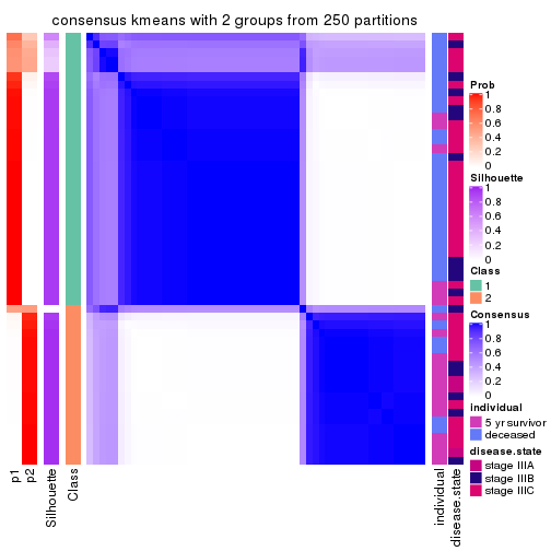
consensus_heatmap(res, k = 3)
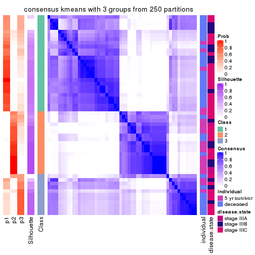
consensus_heatmap(res, k = 4)
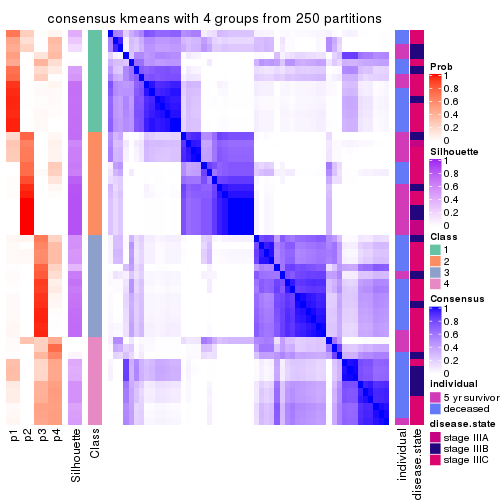
consensus_heatmap(res, k = 5)
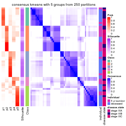
consensus_heatmap(res, k = 6)
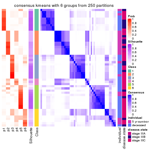
Heatmaps for the membership of samples in all partitions to see how consistent they are:
membership_heatmap(res, k = 2)
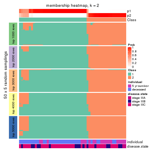
membership_heatmap(res, k = 3)
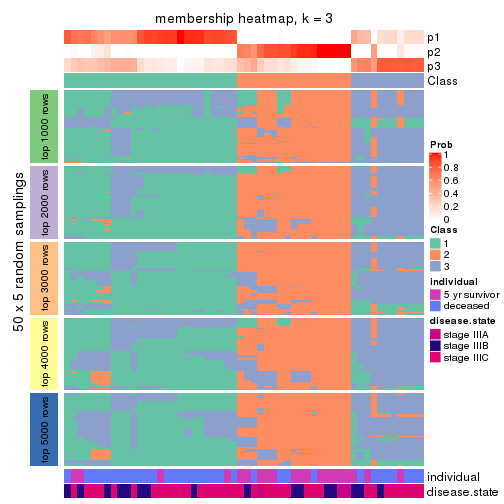
membership_heatmap(res, k = 4)
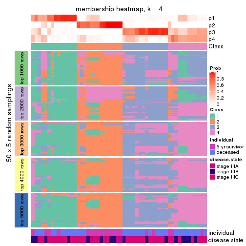
membership_heatmap(res, k = 5)
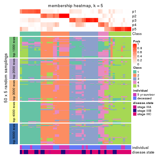
membership_heatmap(res, k = 6)
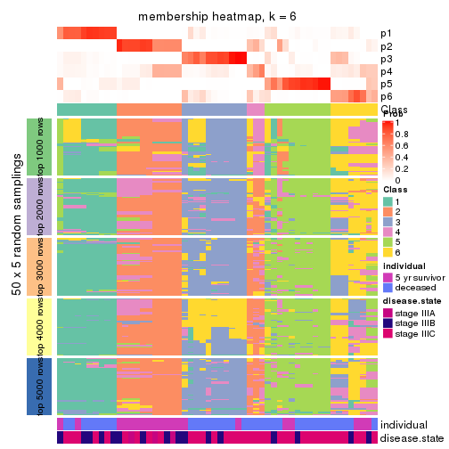
As soon as we have had the classes for columns, we can look for signatures which are significantly different between classes which can be candidate marks for certain classes. Following are the heatmaps for signatures.
Signature heatmaps where rows are scaled:
get_signatures(res, k = 2)
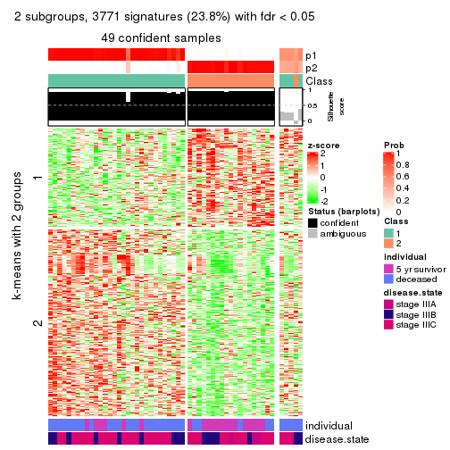
get_signatures(res, k = 3)
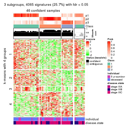
get_signatures(res, k = 4)
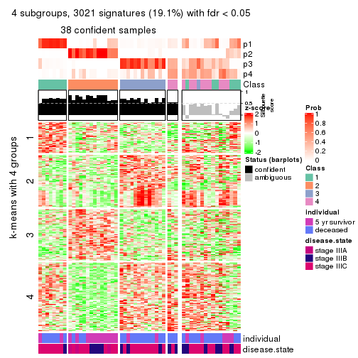
get_signatures(res, k = 5)
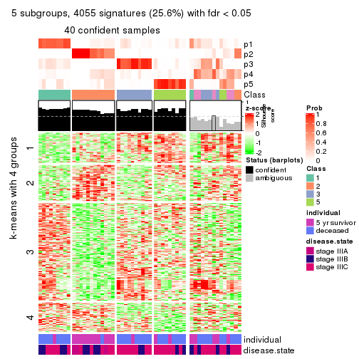
get_signatures(res, k = 6)
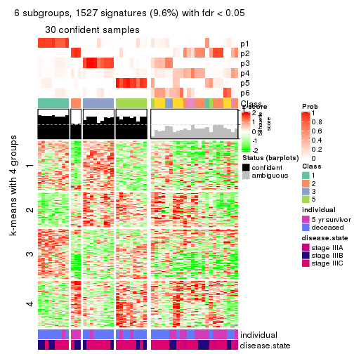
Signature heatmaps where rows are not scaled:
get_signatures(res, k = 2, scale_rows = FALSE)
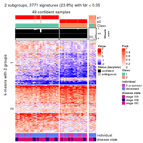
get_signatures(res, k = 3, scale_rows = FALSE)
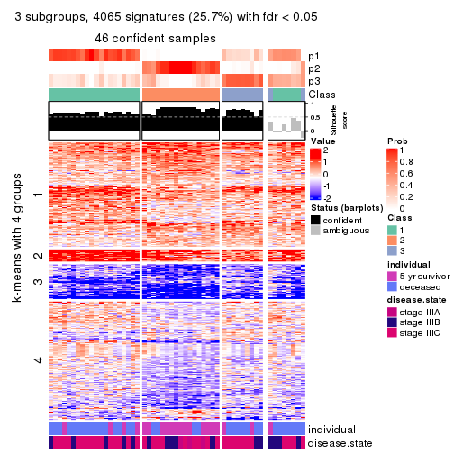
get_signatures(res, k = 4, scale_rows = FALSE)
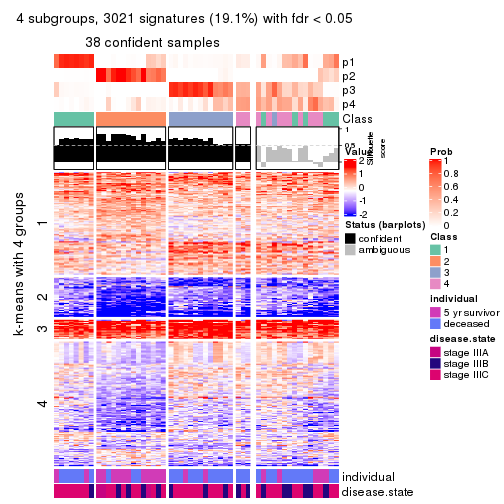
get_signatures(res, k = 5, scale_rows = FALSE)
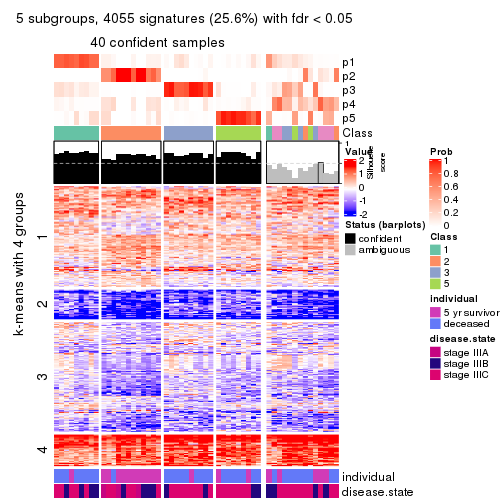
get_signatures(res, k = 6, scale_rows = FALSE)
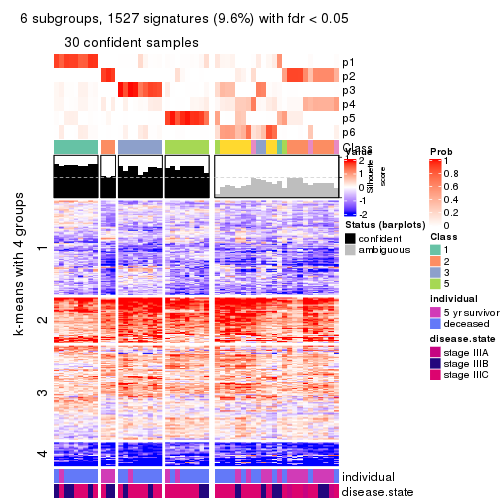
Compare the overlap of signatures from different k:
compare_signatures(res)
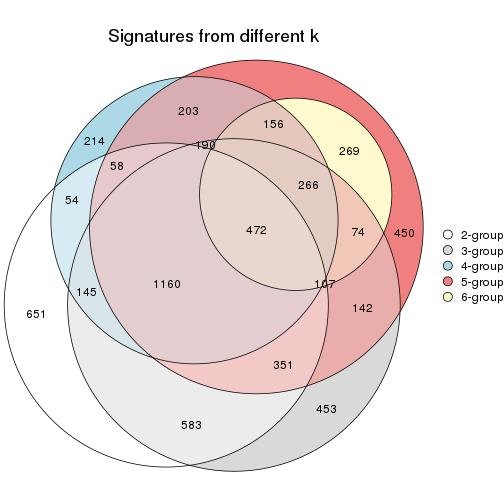
get_signature() returns a data frame invisibly. TO get the list of signatures, the function
call should be assigned to a variable explicitly. In following code, if plot argument is set
to FALSE, no heatmap is plotted while only the differential analysis is performed.
# code only for demonstration
tb = get_signature(res, k = ..., plot = FALSE)
An example of the output of tb is:
#>   which_row         fdr    mean_1    mean_2 scaled_mean_1 scaled_mean_2 km
#> 1        38 0.042760348  8.373488  9.131774    -0.5533452     0.5164555  1
#> 2        40 0.018707592  7.106213  8.469186    -0.6173731     0.5762149  1
#> 3        55 0.019134737 10.221463 11.207825    -0.6159697     0.5749050  1
#> 4        59 0.006059896  5.921854  7.869574    -0.6899429     0.6439467  1
#> 5        60 0.018055526  8.928898 10.211722    -0.6204761     0.5791110  1
#> 6        98 0.009384629 15.714769 14.887706     0.6635654    -0.6193277  2
...
The columns in tb are:
which_row: row indices corresponding to the input matrix.fdr: FDR for the differential test. mean_x: The mean value in group x.scaled_mean_x: The mean value in group x after rows are scaled.km: Row groups if k-means clustering is applied to rows.UMAP plot which shows how samples are separated.
dimension_reduction(res, k = 2, method = "UMAP")
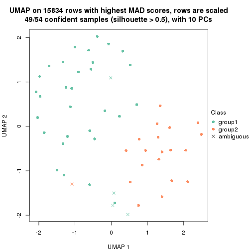
dimension_reduction(res, k = 3, method = "UMAP")
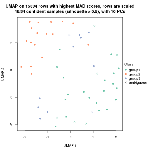
dimension_reduction(res, k = 4, method = "UMAP")
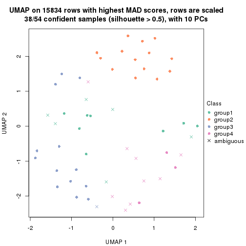
dimension_reduction(res, k = 5, method = "UMAP")
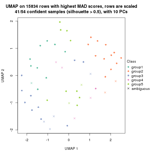
dimension_reduction(res, k = 6, method = "UMAP")
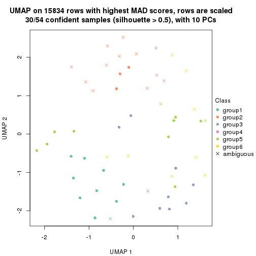
Following heatmap shows how subgroups are split when increasing k:
collect_classes(res)
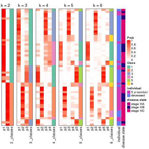
Test correlation between subgroups and known annotations. If the known annotation is numeric, one-way ANOVA test is applied, and if the known annotation is discrete, chi-squared contingency table test is applied.
test_to_known_factors(res)
#>             n individual(p) disease.state(p) k
#> MAD:kmeans 49      0.000610           0.0799 2
#> MAD:kmeans 46      0.001024           0.1923 3
#> MAD:kmeans 38      0.002022           0.1480 4
#> MAD:kmeans 41      0.000121           0.2202 5
#> MAD:kmeans 30      0.009901           0.3916 6
If matrix rows can be associated to genes, consider to use functional_enrichment(res,
...) to perform function enrichment for the signature genes. See this vignette for more detailed explanations.
The object with results only for a single top-value method and a single partition method can be extracted as:
res = res_list["MAD", "skmeans"]
# you can also extract it by
# res = res_list["MAD:skmeans"]
A summary of res and all the functions that can be applied to it:
res
#> A 'ConsensusPartition' object with k = 2, 3, 4, 5, 6.
#>   On a matrix with 15834 rows and 54 columns.
#>   Top rows (1000, 2000, 3000, 4000, 5000) are extracted by 'MAD' method.
#>   Subgroups are detected by 'skmeans' method.
#>   Performed in total 1250 partitions by row resampling.
#>   Best k for subgroups seems to be 2.
#>
#> Following methods can be applied to this 'ConsensusPartition' object:
#>  [1] "cola_report"             "collect_classes"         "collect_plots"
#>  [4] "collect_stats"           "colnames"                "compare_signatures"
#>  [7] "consensus_heatmap"       "dimension_reduction"     "functional_enrichment"
#> [10] "get_anno_col"            "get_anno"                "get_classes"
#> [13] "get_consensus"           "get_matrix"              "get_membership"
#> [16] "get_param"               "get_signatures"          "get_stats"
#> [19] "is_best_k"               "is_stable_k"             "membership_heatmap"
#> [22] "ncol"                    "nrow"                    "plot_ecdf"
#> [25] "rownames"                "select_partition_number" "show"
#> [28] "suggest_best_k"          "test_to_known_factors"
collect_plots() function collects all the plots made from res for all k (number of partitions)
into one single page to provide an easy and fast comparison between different k.
collect_plots(res)
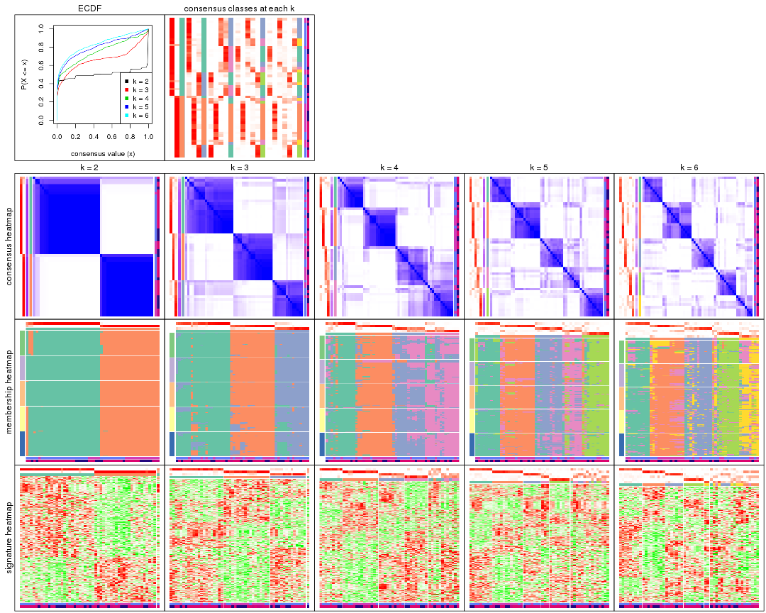
The plots are:
k and the heatmap of
predicted classes for each k.k.k.k.All the plots in panels can be made by individual functions and they are plotted later in this section.
select_partition_number() produces several plots showing different
statistics for choosing “optimized” k. There are following statistics:
k;k, the area increased is defined as \(A_k - A_{k-1}\).The detailed explanations of these statistics can be found in the cola vignette.
Generally speaking, lower PAC score, higher mean silhouette score or higher
concordance corresponds to better partition. Rand index and Jaccard index
measure how similar the current partition is compared to partition with k-1.
If they are too similar, we won't accept k is better than k-1.
select_partition_number(res)
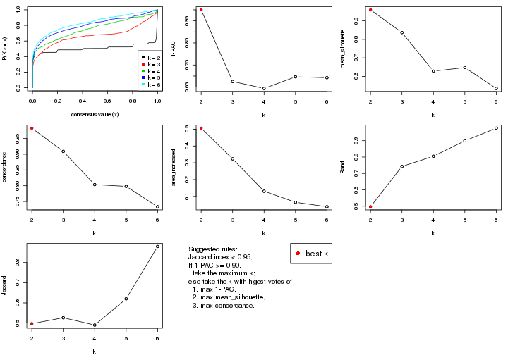
The numeric values for all these statistics can be obtained by get_stats().
get_stats(res)
#>   k 1-PAC mean_silhouette concordance area_increased  Rand Jaccard
#> 2 2 1.000           0.960       0.983         0.5060 0.497   0.497
#> 3 3 0.675           0.837       0.909         0.3235 0.743   0.526
#> 4 4 0.644           0.629       0.804         0.1309 0.805   0.490
#> 5 5 0.696           0.648       0.798         0.0651 0.899   0.620
#> 6 6 0.693           0.535       0.733         0.0385 0.976   0.879
suggest_best_k() suggests the best \(k\) based on these statistics. The rules are as follows:
suggest_best_k(res)
#> [1] 2
Following shows the table of the partitions (You need to click the show/hide
code output link to see it). The membership matrix (columns with name p*)
is inferred by
clue::cl_consensus()
function with the SE method. Basically the value in the membership matrix
represents the probability to belong to a certain group. The finall class
label for an item is determined with the group with highest probability it
belongs to.
In get_classes() function, the entropy is calculated from the membership
matrix and the silhouette score is calculated from the consensus matrix.
cbind(get_classes(res, k = 2), get_membership(res, k = 2))
#>           class entropy silhouette    p1    p2
#> GSM311939     2  0.0000      0.996 0.000 1.000
#> GSM311963     2  0.0000      0.996 0.000 1.000
#> GSM311973     2  0.0000      0.996 0.000 1.000
#> GSM311940     2  0.0000      0.996 0.000 1.000
#> GSM311953     2  0.0000      0.996 0.000 1.000
#> GSM311974     2  0.0000      0.996 0.000 1.000
#> GSM311975     1  0.0000      0.970 1.000 0.000
#> GSM311977     2  0.0000      0.996 0.000 1.000
#> GSM311982     1  0.0000      0.970 1.000 0.000
#> GSM311990     2  0.0000      0.996 0.000 1.000
#> GSM311943     1  0.0000      0.970 1.000 0.000
#> GSM311944     1  0.0000      0.970 1.000 0.000
#> GSM311946     2  0.0000      0.996 0.000 1.000
#> GSM311956     2  0.0000      0.996 0.000 1.000
#> GSM311967     2  0.0000      0.996 0.000 1.000
#> GSM311968     2  0.0000      0.996 0.000 1.000
#> GSM311972     1  0.0000      0.970 1.000 0.000
#> GSM311980     2  0.0000      0.996 0.000 1.000
#> GSM311981     1  0.0672      0.965 0.992 0.008
#> GSM311988     2  0.0000      0.996 0.000 1.000
#> GSM311957     1  0.1184      0.959 0.984 0.016
#> GSM311960     2  0.0000      0.996 0.000 1.000
#> GSM311971     1  0.7219      0.758 0.800 0.200
#> GSM311976     1  0.0000      0.970 1.000 0.000
#> GSM311978     1  0.0000      0.970 1.000 0.000
#> GSM311979     1  0.0000      0.970 1.000 0.000
#> GSM311983     1  0.0000      0.970 1.000 0.000
#> GSM311986     2  0.4022      0.909 0.080 0.920
#> GSM311991     1  0.0000      0.970 1.000 0.000
#> GSM311938     2  0.0000      0.996 0.000 1.000
#> GSM311941     1  0.0000      0.970 1.000 0.000
#> GSM311942     2  0.0672      0.989 0.008 0.992
#> GSM311945     1  0.1184      0.959 0.984 0.016
#> GSM311947     2  0.0000      0.996 0.000 1.000
#> GSM311948     2  0.0000      0.996 0.000 1.000
#> GSM311949     1  0.0000      0.970 1.000 0.000
#> GSM311950     2  0.0000      0.996 0.000 1.000
#> GSM311951     2  0.0672      0.989 0.008 0.992
#> GSM311952     1  0.0000      0.970 1.000 0.000
#> GSM311954     1  0.0938      0.962 0.988 0.012
#> GSM311955     1  0.0000      0.970 1.000 0.000
#> GSM311958     1  0.0000      0.970 1.000 0.000
#> GSM311959     1  0.0000      0.970 1.000 0.000
#> GSM311961     1  0.0000      0.970 1.000 0.000
#> GSM311962     1  0.0000      0.970 1.000 0.000
#> GSM311964     1  0.0000      0.970 1.000 0.000
#> GSM311965     2  0.0000      0.996 0.000 1.000
#> GSM311966     1  0.0000      0.970 1.000 0.000
#> GSM311969     1  0.0000      0.970 1.000 0.000
#> GSM311970     2  0.0000      0.996 0.000 1.000
#> GSM311984     1  0.0000      0.970 1.000 0.000
#> GSM311985     1  0.0000      0.970 1.000 0.000
#> GSM311987     1  0.9710      0.338 0.600 0.400
#> GSM311989     1  0.7056      0.769 0.808 0.192
cbind(get_classes(res, k = 3), get_membership(res, k = 3))
#>           class entropy silhouette    p1    p2    p3
#> GSM311939     2  0.0000      0.934 0.000 1.000 0.000
#> GSM311963     2  0.0000      0.934 0.000 1.000 0.000
#> GSM311973     2  0.5016      0.753 0.000 0.760 0.240
#> GSM311940     2  0.0000      0.934 0.000 1.000 0.000
#> GSM311953     2  0.1031      0.931 0.000 0.976 0.024
#> GSM311974     2  0.1753      0.923 0.000 0.952 0.048
#> GSM311975     1  0.0424      0.881 0.992 0.000 0.008
#> GSM311977     2  0.0000      0.934 0.000 1.000 0.000
#> GSM311982     3  0.4346      0.812 0.184 0.000 0.816
#> GSM311990     2  0.3192      0.881 0.000 0.888 0.112
#> GSM311943     1  0.1860      0.867 0.948 0.000 0.052
#> GSM311944     3  0.4002      0.820 0.160 0.000 0.840
#> GSM311946     2  0.1031      0.931 0.000 0.976 0.024
#> GSM311956     2  0.3482      0.875 0.000 0.872 0.128
#> GSM311967     2  0.2063      0.914 0.008 0.948 0.044
#> GSM311968     3  0.2959      0.779 0.000 0.100 0.900
#> GSM311972     1  0.2711      0.844 0.912 0.000 0.088
#> GSM311980     2  0.3816      0.860 0.000 0.852 0.148
#> GSM311981     1  0.4015      0.823 0.876 0.096 0.028
#> GSM311988     2  0.0000      0.934 0.000 1.000 0.000
#> GSM311957     3  0.2165      0.864 0.064 0.000 0.936
#> GSM311960     3  0.1289      0.858 0.000 0.032 0.968
#> GSM311971     3  0.5061      0.792 0.208 0.008 0.784
#> GSM311976     1  0.3482      0.812 0.872 0.000 0.128
#> GSM311978     1  0.5497      0.539 0.708 0.000 0.292
#> GSM311979     3  0.4842      0.778 0.224 0.000 0.776
#> GSM311983     1  0.0000      0.882 1.000 0.000 0.000
#> GSM311986     1  0.8556      0.181 0.488 0.416 0.096
#> GSM311991     1  0.0592      0.880 0.988 0.000 0.012
#> GSM311938     2  0.0475      0.932 0.004 0.992 0.004
#> GSM311941     3  0.6228      0.536 0.316 0.012 0.672
#> GSM311942     3  0.0475      0.866 0.004 0.004 0.992
#> GSM311945     3  0.0424      0.870 0.008 0.000 0.992
#> GSM311947     2  0.3619      0.873 0.000 0.864 0.136
#> GSM311948     2  0.4842      0.795 0.000 0.776 0.224
#> GSM311949     1  0.4291      0.748 0.820 0.000 0.180
#> GSM311950     2  0.0237      0.933 0.000 0.996 0.004
#> GSM311951     3  0.0829      0.867 0.004 0.012 0.984
#> GSM311952     1  0.0237      0.882 0.996 0.000 0.004
#> GSM311954     1  0.5656      0.755 0.804 0.128 0.068
#> GSM311955     1  0.0000      0.882 1.000 0.000 0.000
#> GSM311958     1  0.0000      0.882 1.000 0.000 0.000
#> GSM311959     1  0.2846      0.854 0.924 0.020 0.056
#> GSM311961     1  0.0424      0.881 0.992 0.000 0.008
#> GSM311962     1  0.0000      0.882 1.000 0.000 0.000
#> GSM311964     3  0.4796      0.782 0.220 0.000 0.780
#> GSM311965     3  0.0424      0.866 0.000 0.008 0.992
#> GSM311966     1  0.2537      0.849 0.920 0.000 0.080
#> GSM311969     1  0.1860      0.867 0.948 0.000 0.052
#> GSM311970     2  0.0237      0.934 0.000 0.996 0.004
#> GSM311984     1  0.0000      0.882 1.000 0.000 0.000
#> GSM311985     1  0.2711      0.844 0.912 0.000 0.088
#> GSM311987     1  0.6605      0.701 0.752 0.152 0.096
#> GSM311989     3  0.0424      0.870 0.008 0.000 0.992
cbind(get_classes(res, k = 4), get_membership(res, k = 4))
#>           class entropy silhouette    p1    p2    p3    p4
#> GSM311939     2  0.0188     0.8964 0.000 0.996 0.004 0.000
#> GSM311963     2  0.0188     0.8964 0.000 0.996 0.004 0.000
#> GSM311973     2  0.2345     0.8392 0.100 0.900 0.000 0.000
#> GSM311940     2  0.0188     0.8964 0.000 0.996 0.004 0.000
#> GSM311953     2  0.0000     0.8957 0.000 1.000 0.000 0.000
#> GSM311974     2  0.0817     0.8875 0.024 0.976 0.000 0.000
#> GSM311975     3  0.3074     0.6265 0.000 0.000 0.848 0.152
#> GSM311977     2  0.0188     0.8964 0.000 0.996 0.004 0.000
#> GSM311982     4  0.4994     0.1693 0.480 0.000 0.000 0.520
#> GSM311990     2  0.7851     0.0943 0.288 0.400 0.312 0.000
#> GSM311943     3  0.5173     0.6243 0.020 0.000 0.660 0.320
#> GSM311944     1  0.2996     0.7698 0.892 0.000 0.044 0.064
#> GSM311946     2  0.0000     0.8957 0.000 1.000 0.000 0.000
#> GSM311956     2  0.2216     0.8458 0.092 0.908 0.000 0.000
#> GSM311967     3  0.5721    -0.1133 0.016 0.412 0.564 0.008
#> GSM311968     1  0.1284     0.8171 0.964 0.024 0.012 0.000
#> GSM311972     4  0.0592     0.6852 0.000 0.000 0.016 0.984
#> GSM311980     2  0.2216     0.8458 0.092 0.908 0.000 0.000
#> GSM311981     4  0.5336     0.1674 0.004 0.004 0.496 0.496
#> GSM311988     2  0.0188     0.8964 0.000 0.996 0.004 0.000
#> GSM311957     1  0.4508     0.6312 0.780 0.000 0.036 0.184
#> GSM311960     1  0.0188     0.8258 0.996 0.000 0.000 0.004
#> GSM311971     4  0.4935     0.6310 0.200 0.040 0.004 0.756
#> GSM311976     4  0.2089     0.6898 0.028 0.012 0.020 0.940
#> GSM311978     4  0.0524     0.6861 0.008 0.000 0.004 0.988
#> GSM311979     4  0.3982     0.6373 0.220 0.000 0.004 0.776
#> GSM311983     3  0.5119     0.4724 0.004 0.000 0.556 0.440
#> GSM311986     3  0.1543     0.5899 0.008 0.032 0.956 0.004
#> GSM311991     4  0.4522     0.4435 0.000 0.000 0.320 0.680
#> GSM311938     2  0.4365     0.7366 0.000 0.784 0.188 0.028
#> GSM311941     1  0.7458     0.2848 0.508 0.000 0.252 0.240
#> GSM311942     1  0.0188     0.8254 0.996 0.000 0.004 0.000
#> GSM311945     1  0.0188     0.8258 0.996 0.000 0.000 0.004
#> GSM311947     1  0.7250     0.3873 0.504 0.160 0.336 0.000
#> GSM311948     1  0.5024     0.3877 0.632 0.360 0.008 0.000
#> GSM311949     4  0.1109     0.6924 0.028 0.000 0.004 0.968
#> GSM311950     2  0.4040     0.7000 0.000 0.752 0.248 0.000
#> GSM311951     1  0.0188     0.8258 0.996 0.000 0.000 0.004
#> GSM311952     3  0.5004     0.5559 0.004 0.000 0.604 0.392
#> GSM311954     3  0.2773     0.6141 0.004 0.000 0.880 0.116
#> GSM311955     3  0.4624     0.6260 0.000 0.000 0.660 0.340
#> GSM311958     3  0.4998     0.4135 0.000 0.000 0.512 0.488
#> GSM311959     3  0.2714     0.6156 0.004 0.000 0.884 0.112
#> GSM311961     4  0.4872     0.0627 0.004 0.000 0.356 0.640
#> GSM311962     4  0.4790    -0.1472 0.000 0.000 0.380 0.620
#> GSM311964     4  0.3945     0.6394 0.216 0.000 0.004 0.780
#> GSM311965     1  0.0469     0.8237 0.988 0.000 0.012 0.000
#> GSM311966     4  0.0469     0.6852 0.000 0.000 0.012 0.988
#> GSM311969     3  0.4608     0.6385 0.004 0.000 0.692 0.304
#> GSM311970     2  0.0779     0.8913 0.000 0.980 0.016 0.004
#> GSM311984     3  0.4800     0.6167 0.004 0.000 0.656 0.340
#> GSM311985     4  0.0592     0.6852 0.000 0.000 0.016 0.984
#> GSM311987     3  0.2125     0.5952 0.004 0.000 0.920 0.076
#> GSM311989     1  0.0188     0.8258 0.996 0.000 0.000 0.004
cbind(get_classes(res, k = 5), get_membership(res, k = 5))
#>           class entropy silhouette    p1    p2    p3    p4    p5
#> GSM311939     2  0.1205    0.85002 0.000 0.956 0.000 0.040 0.004
#> GSM311963     2  0.0880    0.85292 0.000 0.968 0.000 0.032 0.000
#> GSM311973     2  0.4011    0.79837 0.040 0.832 0.004 0.048 0.076
#> GSM311940     2  0.0880    0.85292 0.000 0.968 0.000 0.032 0.000
#> GSM311953     2  0.1644    0.84463 0.008 0.948 0.004 0.028 0.012
#> GSM311974     2  0.2672    0.83000 0.008 0.900 0.004 0.040 0.048
#> GSM311975     3  0.4525    0.44699 0.016 0.000 0.624 0.360 0.000
#> GSM311977     2  0.0880    0.85292 0.000 0.968 0.000 0.032 0.000
#> GSM311982     1  0.4872    0.22503 0.540 0.000 0.024 0.000 0.436
#> GSM311990     4  0.6141    0.37287 0.000 0.164 0.004 0.572 0.260
#> GSM311943     3  0.1173    0.74429 0.004 0.000 0.964 0.020 0.012
#> GSM311944     5  0.4171    0.66323 0.028 0.000 0.152 0.028 0.792
#> GSM311946     2  0.0451    0.85209 0.000 0.988 0.000 0.004 0.008
#> GSM311956     2  0.3473    0.80660 0.008 0.852 0.004 0.052 0.084
#> GSM311967     4  0.2362    0.58030 0.000 0.076 0.024 0.900 0.000
#> GSM311968     5  0.2173    0.75264 0.012 0.016 0.000 0.052 0.920
#> GSM311972     1  0.3512    0.79889 0.840 0.000 0.088 0.068 0.004
#> GSM311980     2  0.3653    0.80714 0.020 0.848 0.004 0.048 0.080
#> GSM311981     4  0.3255    0.56315 0.100 0.000 0.052 0.848 0.000
#> GSM311988     2  0.1205    0.85002 0.000 0.956 0.000 0.040 0.004
#> GSM311957     5  0.5903    0.49066 0.256 0.008 0.092 0.012 0.632
#> GSM311960     5  0.1877    0.77454 0.052 0.008 0.004 0.004 0.932
#> GSM311971     1  0.2266    0.83351 0.912 0.008 0.016 0.000 0.064
#> GSM311976     1  0.1329    0.83938 0.956 0.000 0.008 0.032 0.004
#> GSM311978     1  0.1830    0.84408 0.924 0.000 0.068 0.000 0.008
#> GSM311979     1  0.2012    0.83635 0.920 0.000 0.020 0.000 0.060
#> GSM311983     3  0.2110    0.74439 0.072 0.000 0.912 0.016 0.000
#> GSM311986     3  0.4886    0.37292 0.000 0.036 0.668 0.288 0.008
#> GSM311991     4  0.5905    0.28522 0.276 0.000 0.144 0.580 0.000
#> GSM311938     2  0.5276    0.27919 0.028 0.568 0.008 0.392 0.004
#> GSM311941     5  0.8029   -0.00722 0.232 0.000 0.116 0.232 0.420
#> GSM311942     5  0.0912    0.77823 0.016 0.000 0.000 0.012 0.972
#> GSM311945     5  0.1357    0.77729 0.048 0.004 0.000 0.000 0.948
#> GSM311947     4  0.5068    0.27056 0.000 0.044 0.000 0.592 0.364
#> GSM311948     5  0.5852   -0.01744 0.008 0.452 0.004 0.060 0.476
#> GSM311949     1  0.1588    0.84524 0.948 0.000 0.028 0.016 0.008
#> GSM311950     2  0.4430    0.21709 0.000 0.540 0.000 0.456 0.004
#> GSM311951     5  0.0404    0.77952 0.012 0.000 0.000 0.000 0.988
#> GSM311952     3  0.1043    0.75215 0.040 0.000 0.960 0.000 0.000
#> GSM311954     4  0.5343    0.49541 0.076 0.000 0.280 0.640 0.004
#> GSM311955     3  0.3085    0.68254 0.032 0.000 0.852 0.116 0.000
#> GSM311958     3  0.5610    0.47766 0.184 0.000 0.640 0.176 0.000
#> GSM311959     4  0.5080    0.46481 0.056 0.000 0.316 0.628 0.000
#> GSM311961     3  0.4390    0.65166 0.156 0.000 0.760 0.084 0.000
#> GSM311962     3  0.4696    0.42152 0.360 0.000 0.616 0.024 0.000
#> GSM311964     1  0.1557    0.83781 0.940 0.000 0.000 0.008 0.052
#> GSM311965     5  0.1644    0.76386 0.004 0.008 0.000 0.048 0.940
#> GSM311966     1  0.3165    0.79794 0.848 0.000 0.116 0.036 0.000
#> GSM311969     3  0.0955    0.73973 0.000 0.000 0.968 0.028 0.004
#> GSM311970     2  0.2873    0.79980 0.016 0.856 0.000 0.128 0.000
#> GSM311984     3  0.1943    0.74646 0.020 0.000 0.924 0.056 0.000
#> GSM311985     1  0.3937    0.77422 0.808 0.000 0.116 0.072 0.004
#> GSM311987     4  0.4870    0.51846 0.040 0.000 0.272 0.680 0.008
#> GSM311989     5  0.1251    0.77866 0.036 0.000 0.000 0.008 0.956
cbind(get_classes(res, k = 6), get_membership(res, k = 6))
#>           class entropy silhouette    p1    p2    p3    p4    p5    p6
#> GSM311939     2  0.0909     0.6725 0.000 0.968 0.000 0.020 0.000 0.012
#> GSM311963     2  0.0405     0.6782 0.000 0.988 0.000 0.004 0.000 0.008
#> GSM311973     2  0.5220     0.4557 0.024 0.540 0.000 0.388 0.048 0.000
#> GSM311940     2  0.0508     0.6772 0.000 0.984 0.000 0.012 0.000 0.004
#> GSM311953     2  0.3265     0.6097 0.000 0.748 0.000 0.248 0.004 0.000
#> GSM311974     2  0.4131     0.5284 0.000 0.624 0.000 0.356 0.020 0.000
#> GSM311975     3  0.6210     0.2992 0.028 0.000 0.512 0.268 0.000 0.192
#> GSM311977     2  0.0146     0.6785 0.000 0.996 0.000 0.004 0.000 0.000
#> GSM311982     1  0.5543     0.0807 0.464 0.000 0.032 0.048 0.452 0.004
#> GSM311990     6  0.7210     0.2950 0.000 0.124 0.000 0.288 0.180 0.408
#> GSM311943     3  0.1440     0.6962 0.004 0.000 0.944 0.004 0.004 0.044
#> GSM311944     5  0.4288     0.6888 0.032 0.000 0.116 0.072 0.776 0.004
#> GSM311946     2  0.2902     0.6355 0.000 0.800 0.000 0.196 0.004 0.000
#> GSM311956     2  0.4709     0.4397 0.000 0.540 0.000 0.412 0.048 0.000
#> GSM311967     6  0.4989     0.3823 0.000 0.072 0.008 0.312 0.000 0.608
#> GSM311968     5  0.3271     0.6508 0.000 0.000 0.000 0.232 0.760 0.008
#> GSM311972     1  0.4561     0.7190 0.748 0.000 0.040 0.084 0.000 0.128
#> GSM311980     2  0.4576     0.4745 0.000 0.560 0.000 0.400 0.040 0.000
#> GSM311981     6  0.4806     0.2578 0.056 0.000 0.004 0.348 0.000 0.592
#> GSM311988     2  0.0622     0.6767 0.000 0.980 0.000 0.012 0.000 0.008
#> GSM311957     5  0.6929     0.3448 0.284 0.000 0.116 0.084 0.496 0.020
#> GSM311960     5  0.3220     0.7567 0.056 0.000 0.000 0.108 0.832 0.004
#> GSM311971     1  0.2373     0.7813 0.908 0.016 0.012 0.024 0.040 0.000
#> GSM311976     1  0.2934     0.7652 0.876 0.004 0.016 0.068 0.008 0.028
#> GSM311978     1  0.2421     0.7888 0.900 0.000 0.052 0.032 0.004 0.012
#> GSM311979     1  0.2068     0.7838 0.916 0.000 0.016 0.020 0.048 0.000
#> GSM311983     3  0.1168     0.6993 0.028 0.000 0.956 0.016 0.000 0.000
#> GSM311986     3  0.5565     0.3931 0.000 0.056 0.604 0.064 0.000 0.276
#> GSM311991     4  0.7021    -0.4150 0.188 0.000 0.084 0.368 0.000 0.360
#> GSM311938     2  0.4602     0.2219 0.008 0.600 0.004 0.024 0.000 0.364
#> GSM311941     6  0.7228     0.2642 0.140 0.000 0.072 0.036 0.280 0.472
#> GSM311942     5  0.0922     0.8052 0.000 0.000 0.004 0.024 0.968 0.004
#> GSM311945     5  0.1534     0.8068 0.016 0.000 0.004 0.032 0.944 0.004
#> GSM311947     6  0.6667     0.2934 0.000 0.036 0.000 0.340 0.236 0.388
#> GSM311948     4  0.6264    -0.3313 0.000 0.308 0.000 0.408 0.276 0.008
#> GSM311949     1  0.2144     0.7890 0.912 0.004 0.032 0.048 0.000 0.004
#> GSM311950     2  0.5443     0.2299 0.000 0.572 0.000 0.244 0.000 0.184
#> GSM311951     5  0.0603     0.8109 0.000 0.000 0.004 0.016 0.980 0.000
#> GSM311952     3  0.1088     0.7014 0.016 0.000 0.960 0.000 0.000 0.024
#> GSM311954     6  0.2848     0.5217 0.036 0.000 0.104 0.004 0.000 0.856
#> GSM311955     3  0.3957     0.5215 0.020 0.000 0.696 0.004 0.000 0.280
#> GSM311958     3  0.6881     0.2145 0.208 0.000 0.408 0.064 0.000 0.320
#> GSM311959     6  0.3261     0.4928 0.024 0.000 0.144 0.012 0.000 0.820
#> GSM311961     3  0.4283     0.6176 0.104 0.000 0.776 0.072 0.000 0.048
#> GSM311962     3  0.5772     0.1772 0.376 0.000 0.500 0.024 0.000 0.100
#> GSM311964     1  0.2959     0.7643 0.864 0.000 0.004 0.072 0.052 0.008
#> GSM311965     5  0.2491     0.7634 0.000 0.000 0.000 0.112 0.868 0.020
#> GSM311966     1  0.4070     0.7480 0.796 0.000 0.056 0.040 0.004 0.104
#> GSM311969     3  0.1753     0.6875 0.000 0.000 0.912 0.004 0.000 0.084
#> GSM311970     2  0.3564     0.5709 0.008 0.772 0.000 0.200 0.000 0.020
#> GSM311984     3  0.1659     0.6939 0.008 0.004 0.940 0.028 0.000 0.020
#> GSM311985     1  0.4750     0.7014 0.728 0.000 0.056 0.060 0.000 0.156
#> GSM311987     6  0.2547     0.5267 0.016 0.000 0.112 0.004 0.000 0.868
#> GSM311989     5  0.1534     0.8080 0.016 0.000 0.004 0.032 0.944 0.004
Heatmaps for the consensus matrix. It visualizes the probability of two samples to be in a same group.
consensus_heatmap(res, k = 2)
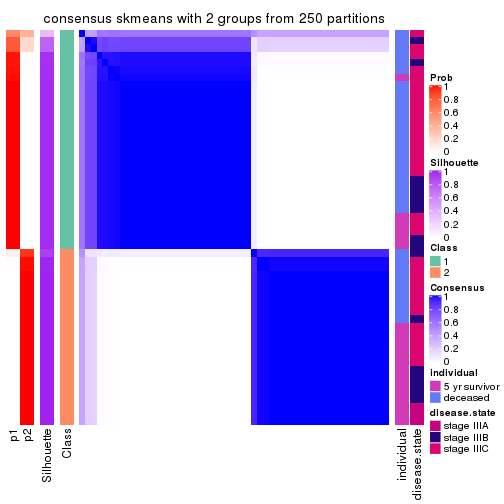
consensus_heatmap(res, k = 3)
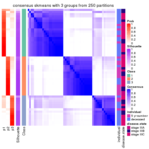
consensus_heatmap(res, k = 4)
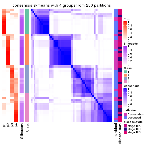
consensus_heatmap(res, k = 5)
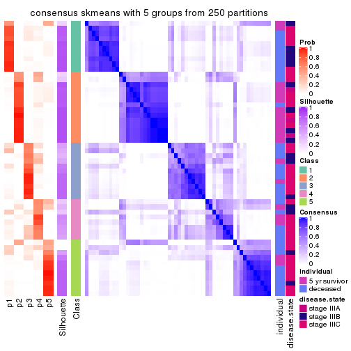
consensus_heatmap(res, k = 6)
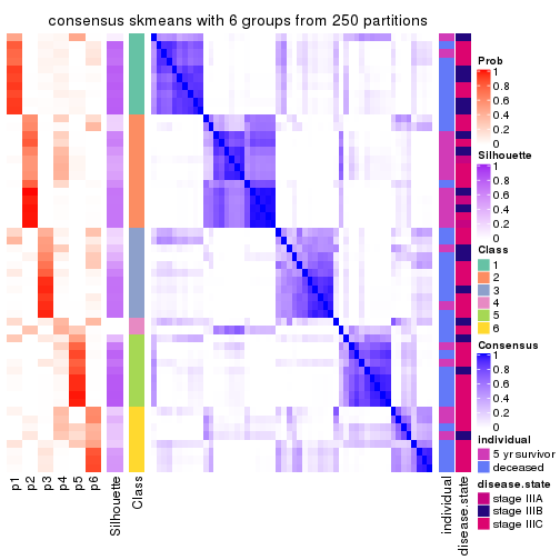
Heatmaps for the membership of samples in all partitions to see how consistent they are:
membership_heatmap(res, k = 2)
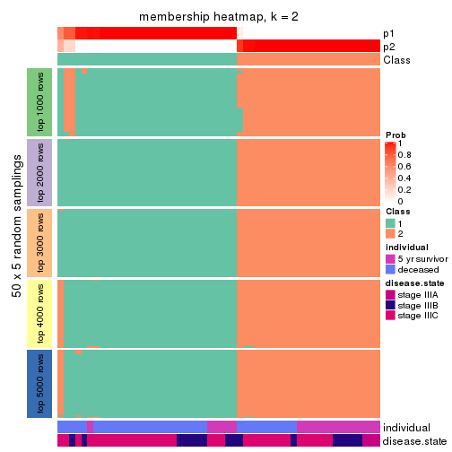
membership_heatmap(res, k = 3)
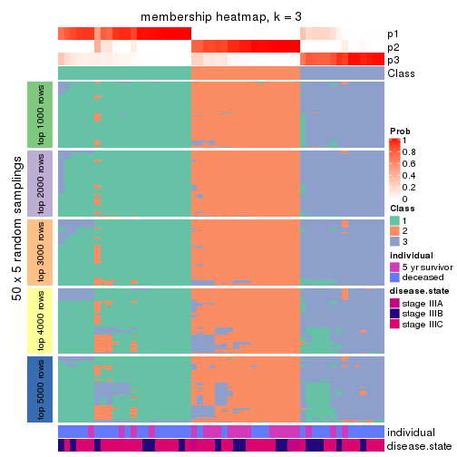
membership_heatmap(res, k = 4)
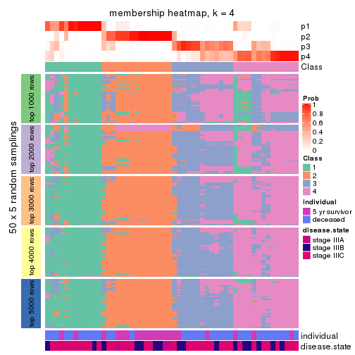
membership_heatmap(res, k = 5)
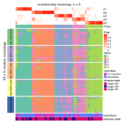
membership_heatmap(res, k = 6)
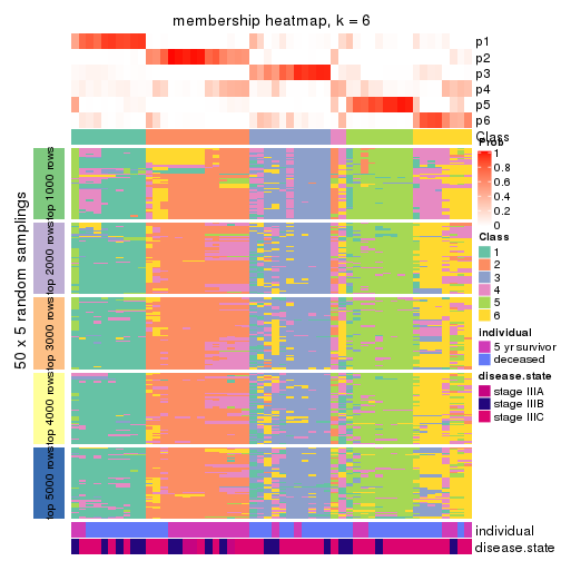
As soon as we have had the classes for columns, we can look for signatures which are significantly different between classes which can be candidate marks for certain classes. Following are the heatmaps for signatures.
Signature heatmaps where rows are scaled:
get_signatures(res, k = 2)
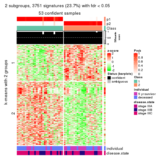
get_signatures(res, k = 3)
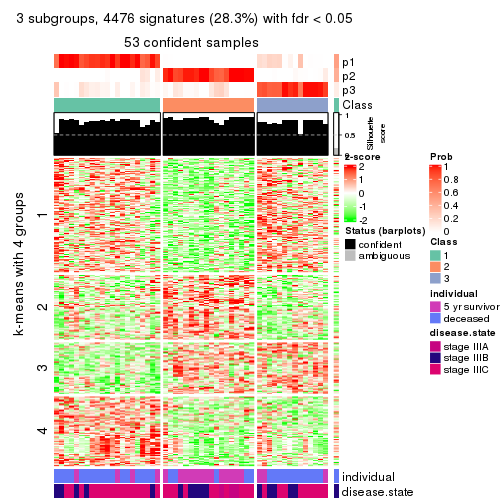
get_signatures(res, k = 4)
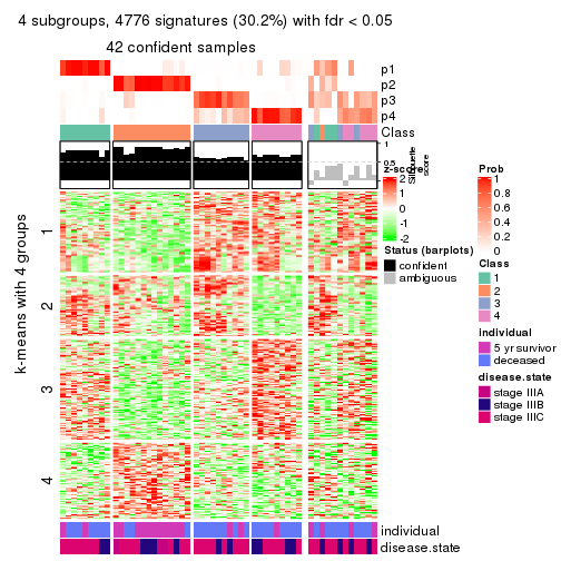
get_signatures(res, k = 5)
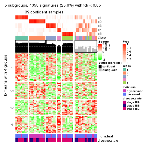
get_signatures(res, k = 6)
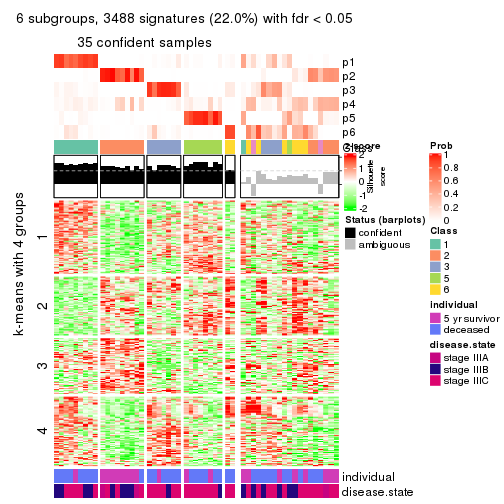
Signature heatmaps where rows are not scaled:
get_signatures(res, k = 2, scale_rows = FALSE)
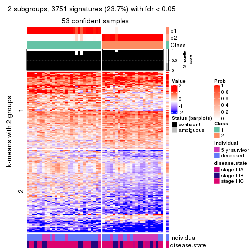
get_signatures(res, k = 3, scale_rows = FALSE)
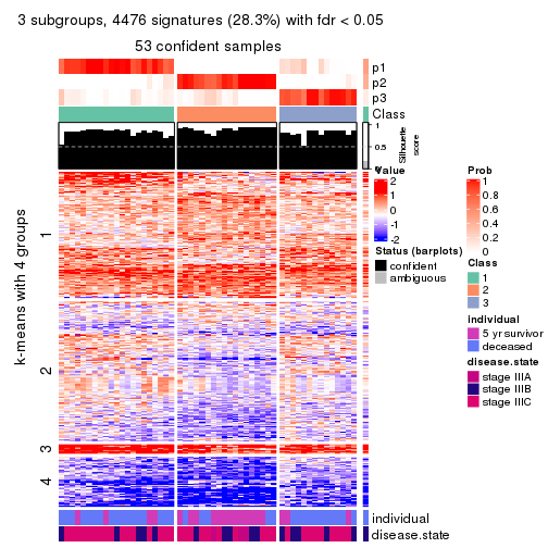
get_signatures(res, k = 4, scale_rows = FALSE)
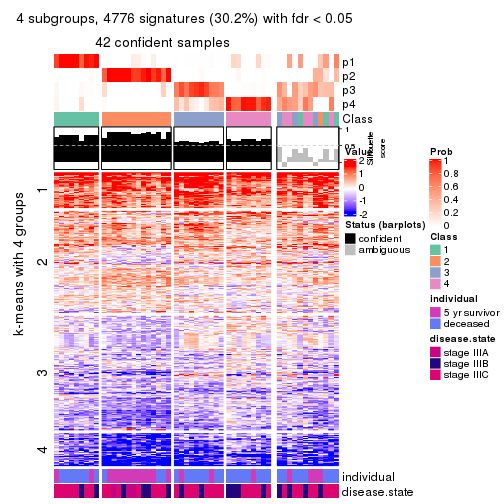
get_signatures(res, k = 5, scale_rows = FALSE)
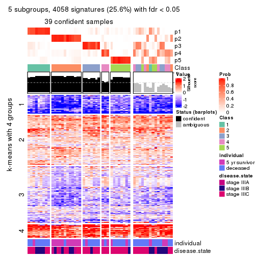
get_signatures(res, k = 6, scale_rows = FALSE)
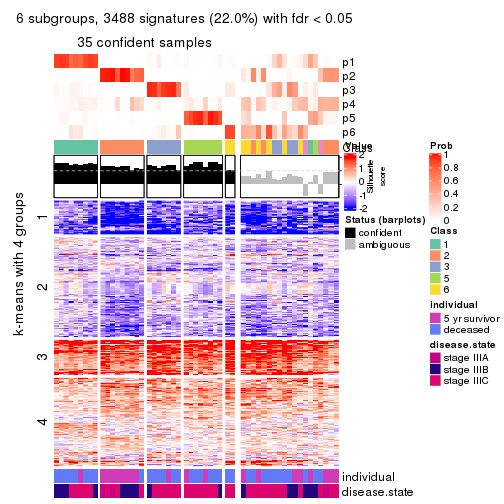
Compare the overlap of signatures from different k:
compare_signatures(res)
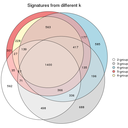
get_signature() returns a data frame invisibly. TO get the list of signatures, the function
call should be assigned to a variable explicitly. In following code, if plot argument is set
to FALSE, no heatmap is plotted while only the differential analysis is performed.
# code only for demonstration
tb = get_signature(res, k = ..., plot = FALSE)
An example of the output of tb is:
#>   which_row         fdr    mean_1    mean_2 scaled_mean_1 scaled_mean_2 km
#> 1        38 0.042760348  8.373488  9.131774    -0.5533452     0.5164555  1
#> 2        40 0.018707592  7.106213  8.469186    -0.6173731     0.5762149  1
#> 3        55 0.019134737 10.221463 11.207825    -0.6159697     0.5749050  1
#> 4        59 0.006059896  5.921854  7.869574    -0.6899429     0.6439467  1
#> 5        60 0.018055526  8.928898 10.211722    -0.6204761     0.5791110  1
#> 6        98 0.009384629 15.714769 14.887706     0.6635654    -0.6193277  2
...
The columns in tb are:
which_row: row indices corresponding to the input matrix.fdr: FDR for the differential test. mean_x: The mean value in group x.scaled_mean_x: The mean value in group x after rows are scaled.km: Row groups if k-means clustering is applied to rows.UMAP plot which shows how samples are separated.
dimension_reduction(res, k = 2, method = "UMAP")
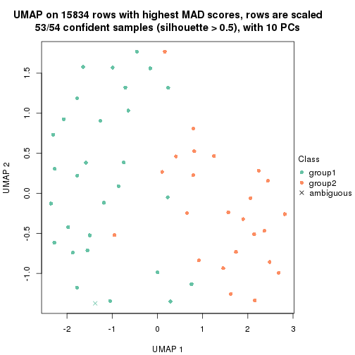
dimension_reduction(res, k = 3, method = "UMAP")
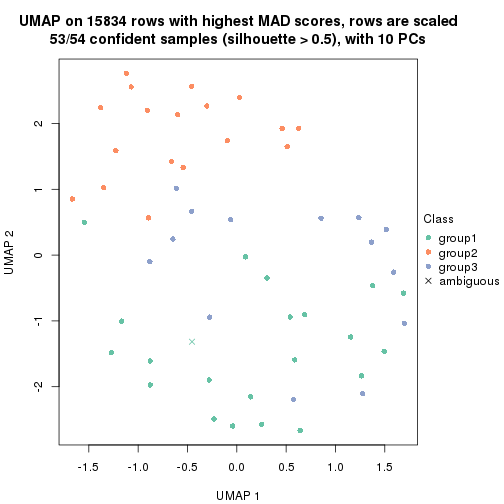
dimension_reduction(res, k = 4, method = "UMAP")
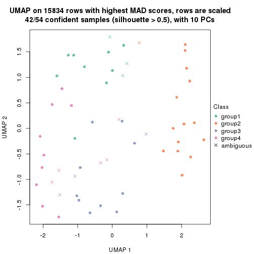
dimension_reduction(res, k = 5, method = "UMAP")
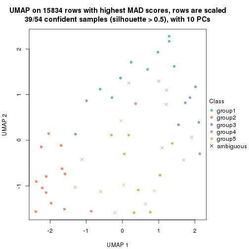
dimension_reduction(res, k = 6, method = "UMAP")
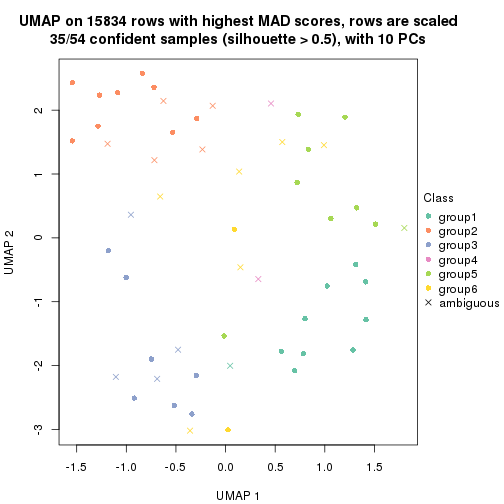
Following heatmap shows how subgroups are split when increasing k:
collect_classes(res)
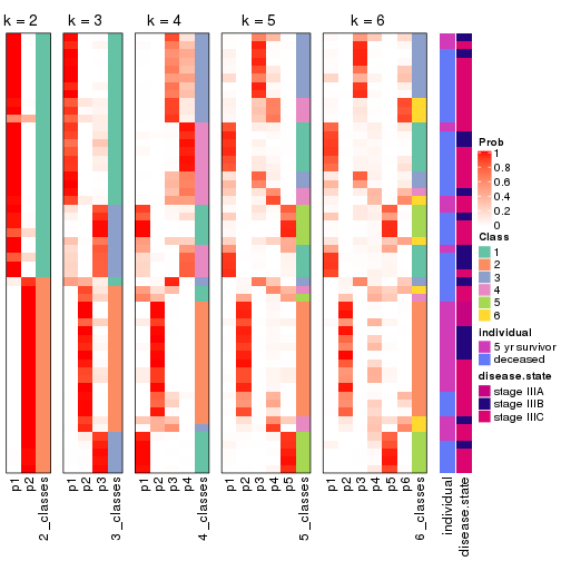
Test correlation between subgroups and known annotations. If the known annotation is numeric, one-way ANOVA test is applied, and if the known annotation is discrete, chi-squared contingency table test is applied.
test_to_known_factors(res)
#>              n individual(p) disease.state(p) k
#> MAD:skmeans 53      0.011419            0.144 2
#> MAD:skmeans 53      0.000999            0.142 3
#> MAD:skmeans 42      0.001945            0.212 4
#> MAD:skmeans 39      0.000668            0.126 5
#> MAD:skmeans 35      0.002263            0.147 6
If matrix rows can be associated to genes, consider to use functional_enrichment(res,
...) to perform function enrichment for the signature genes. See this vignette for more detailed explanations.
The object with results only for a single top-value method and a single partition method can be extracted as:
res = res_list["MAD", "pam"]
# you can also extract it by
# res = res_list["MAD:pam"]
A summary of res and all the functions that can be applied to it:
res
#> A 'ConsensusPartition' object with k = 2, 3, 4, 5, 6.
#>   On a matrix with 15834 rows and 54 columns.
#>   Top rows (1000, 2000, 3000, 4000, 5000) are extracted by 'MAD' method.
#>   Subgroups are detected by 'pam' method.
#>   Performed in total 1250 partitions by row resampling.
#>   Best k for subgroups seems to be 2.
#>
#> Following methods can be applied to this 'ConsensusPartition' object:
#>  [1] "cola_report"             "collect_classes"         "collect_plots"
#>  [4] "collect_stats"           "colnames"                "compare_signatures"
#>  [7] "consensus_heatmap"       "dimension_reduction"     "functional_enrichment"
#> [10] "get_anno_col"            "get_anno"                "get_classes"
#> [13] "get_consensus"           "get_matrix"              "get_membership"
#> [16] "get_param"               "get_signatures"          "get_stats"
#> [19] "is_best_k"               "is_stable_k"             "membership_heatmap"
#> [22] "ncol"                    "nrow"                    "plot_ecdf"
#> [25] "rownames"                "select_partition_number" "show"
#> [28] "suggest_best_k"          "test_to_known_factors"
collect_plots() function collects all the plots made from res for all k (number of partitions)
into one single page to provide an easy and fast comparison between different k.
collect_plots(res)
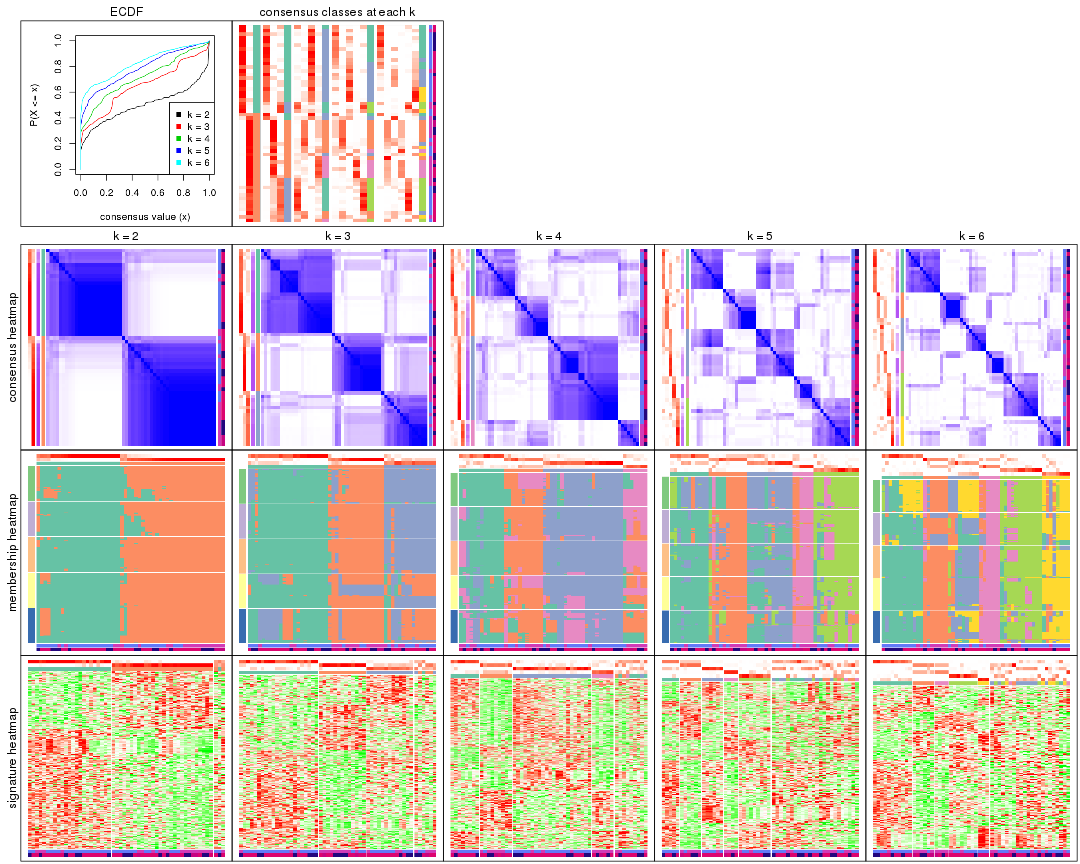
The plots are:
k and the heatmap of
predicted classes for each k.k.k.k.All the plots in panels can be made by individual functions and they are plotted later in this section.
select_partition_number() produces several plots showing different
statistics for choosing “optimized” k. There are following statistics:
k;k, the area increased is defined as \(A_k - A_{k-1}\).The detailed explanations of these statistics can be found in the cola vignette.
Generally speaking, lower PAC score, higher mean silhouette score or higher
concordance corresponds to better partition. Rand index and Jaccard index
measure how similar the current partition is compared to partition with k-1.
If they are too similar, we won't accept k is better than k-1.
select_partition_number(res)
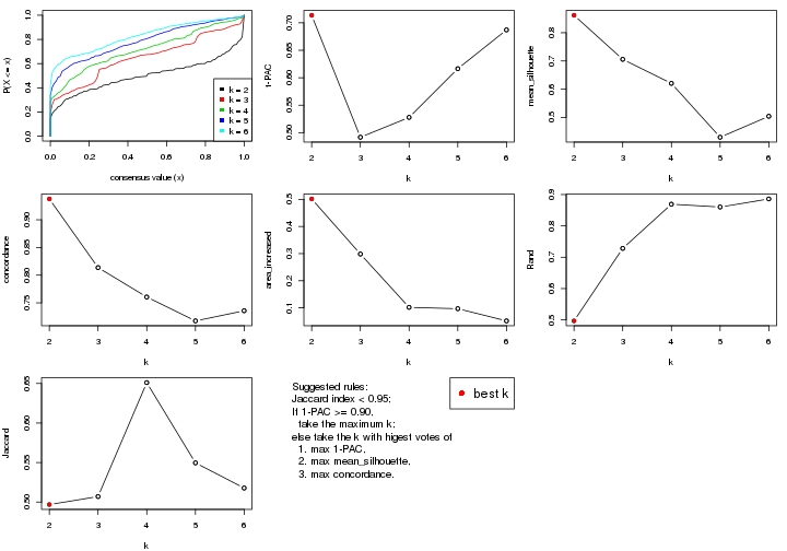
The numeric values for all these statistics can be obtained by get_stats().
get_stats(res)
#>   k 1-PAC mean_silhouette concordance area_increased  Rand Jaccard
#> 2 2 0.714           0.862       0.938         0.5016 0.497   0.497
#> 3 3 0.492           0.706       0.814         0.2984 0.728   0.507
#> 4 4 0.528           0.621       0.761         0.1019 0.869   0.651
#> 5 5 0.616           0.430       0.717         0.0969 0.860   0.550
#> 6 6 0.687           0.504       0.736         0.0520 0.886   0.518
suggest_best_k() suggests the best \(k\) based on these statistics. The rules are as follows:
suggest_best_k(res)
#> [1] 2
Following shows the table of the partitions (You need to click the show/hide
code output link to see it). The membership matrix (columns with name p*)
is inferred by
clue::cl_consensus()
function with the SE method. Basically the value in the membership matrix
represents the probability to belong to a certain group. The finall class
label for an item is determined with the group with highest probability it
belongs to.
In get_classes() function, the entropy is calculated from the membership
matrix and the silhouette score is calculated from the consensus matrix.
cbind(get_classes(res, k = 2), get_membership(res, k = 2))
#>           class entropy silhouette    p1    p2
#> GSM311939     2  0.0000     0.9293 0.000 1.000
#> GSM311963     2  0.0000     0.9293 0.000 1.000
#> GSM311973     2  0.0000     0.9293 0.000 1.000
#> GSM311940     2  0.0000     0.9293 0.000 1.000
#> GSM311953     2  0.0000     0.9293 0.000 1.000
#> GSM311974     2  0.0000     0.9293 0.000 1.000
#> GSM311975     2  0.5737     0.8332 0.136 0.864
#> GSM311977     2  0.0000     0.9293 0.000 1.000
#> GSM311982     1  0.3431     0.8939 0.936 0.064
#> GSM311990     2  0.0376     0.9284 0.004 0.996
#> GSM311943     1  0.0000     0.9322 1.000 0.000
#> GSM311944     1  0.1633     0.9206 0.976 0.024
#> GSM311946     2  0.0000     0.9293 0.000 1.000
#> GSM311956     2  0.0000     0.9293 0.000 1.000
#> GSM311967     2  0.0000     0.9293 0.000 1.000
#> GSM311968     2  0.0376     0.9284 0.004 0.996
#> GSM311972     1  0.0000     0.9322 1.000 0.000
#> GSM311980     2  0.0000     0.9293 0.000 1.000
#> GSM311981     2  0.9850     0.2639 0.428 0.572
#> GSM311988     2  0.0000     0.9293 0.000 1.000
#> GSM311957     2  0.6531     0.8004 0.168 0.832
#> GSM311960     2  0.2236     0.9145 0.036 0.964
#> GSM311971     1  0.9393     0.4462 0.644 0.356
#> GSM311976     1  0.0376     0.9306 0.996 0.004
#> GSM311978     1  0.0000     0.9322 1.000 0.000
#> GSM311979     1  0.0000     0.9322 1.000 0.000
#> GSM311983     1  0.2948     0.9014 0.948 0.052
#> GSM311986     2  0.1414     0.9215 0.020 0.980
#> GSM311991     1  0.3584     0.8933 0.932 0.068
#> GSM311938     2  0.0672     0.9267 0.008 0.992
#> GSM311941     1  0.0000     0.9322 1.000 0.000
#> GSM311942     2  0.6048     0.8358 0.148 0.852
#> GSM311945     2  0.7219     0.7755 0.200 0.800
#> GSM311947     2  0.0938     0.9256 0.012 0.988
#> GSM311948     2  0.0000     0.9293 0.000 1.000
#> GSM311949     1  0.2423     0.9099 0.960 0.040
#> GSM311950     2  0.0000     0.9293 0.000 1.000
#> GSM311951     2  0.4562     0.8795 0.096 0.904
#> GSM311952     1  0.8861     0.5878 0.696 0.304
#> GSM311954     1  0.0000     0.9322 1.000 0.000
#> GSM311955     1  0.0000     0.9322 1.000 0.000
#> GSM311958     1  0.0000     0.9322 1.000 0.000
#> GSM311959     1  0.0000     0.9322 1.000 0.000
#> GSM311961     2  1.0000     0.0424 0.496 0.504
#> GSM311962     1  0.0000     0.9322 1.000 0.000
#> GSM311964     1  0.0000     0.9322 1.000 0.000
#> GSM311965     2  0.4022     0.8889 0.080 0.920
#> GSM311966     1  0.0000     0.9322 1.000 0.000
#> GSM311969     1  0.0000     0.9322 1.000 0.000
#> GSM311970     2  0.0000     0.9293 0.000 1.000
#> GSM311984     1  0.8327     0.6617 0.736 0.264
#> GSM311985     1  0.0000     0.9322 1.000 0.000
#> GSM311987     1  0.8016     0.6669 0.756 0.244
#> GSM311989     2  0.5059     0.8679 0.112 0.888
cbind(get_classes(res, k = 3), get_membership(res, k = 3))
#>           class entropy silhouette    p1    p2    p3
#> GSM311939     2  0.0000      0.854 0.000 1.000 0.000
#> GSM311963     2  0.0000      0.854 0.000 1.000 0.000
#> GSM311973     2  0.6045      0.148 0.000 0.620 0.380
#> GSM311940     2  0.0000      0.854 0.000 1.000 0.000
#> GSM311953     2  0.0592      0.851 0.000 0.988 0.012
#> GSM311974     2  0.1964      0.813 0.000 0.944 0.056
#> GSM311975     1  0.5325      0.638 0.748 0.248 0.004
#> GSM311977     2  0.0000      0.854 0.000 1.000 0.000
#> GSM311982     3  0.6045      0.403 0.380 0.000 0.620
#> GSM311990     3  0.5560      0.703 0.000 0.300 0.700
#> GSM311943     1  0.4842      0.782 0.776 0.000 0.224
#> GSM311944     3  0.3038      0.642 0.104 0.000 0.896
#> GSM311946     2  0.0592      0.851 0.000 0.988 0.012
#> GSM311956     2  0.0592      0.851 0.000 0.988 0.012
#> GSM311967     2  0.5285      0.560 0.004 0.752 0.244
#> GSM311968     3  0.5058      0.764 0.000 0.244 0.756
#> GSM311972     1  0.1529      0.818 0.960 0.000 0.040
#> GSM311980     2  0.5678      0.355 0.000 0.684 0.316
#> GSM311981     3  0.6654     -0.126 0.008 0.456 0.536
#> GSM311988     2  0.0000      0.854 0.000 1.000 0.000
#> GSM311957     3  0.9141      0.599 0.212 0.244 0.544
#> GSM311960     3  0.5502      0.769 0.008 0.248 0.744
#> GSM311971     1  0.7569      0.506 0.668 0.240 0.092
#> GSM311976     1  0.0237      0.831 0.996 0.000 0.004
#> GSM311978     1  0.0237      0.831 0.996 0.000 0.004
#> GSM311979     1  0.4399      0.668 0.812 0.000 0.188
#> GSM311983     1  0.0000      0.831 1.000 0.000 0.000
#> GSM311986     2  0.7980      0.245 0.356 0.572 0.072
#> GSM311991     1  0.0237      0.831 0.996 0.004 0.000
#> GSM311938     2  0.2845      0.791 0.068 0.920 0.012
#> GSM311941     3  0.3038      0.582 0.104 0.000 0.896
#> GSM311942     3  0.5420      0.771 0.008 0.240 0.752
#> GSM311945     3  0.5461      0.771 0.008 0.244 0.748
#> GSM311947     3  0.6057      0.699 0.004 0.340 0.656
#> GSM311948     3  0.5785      0.702 0.000 0.332 0.668
#> GSM311949     1  0.2550      0.819 0.932 0.056 0.012
#> GSM311950     2  0.0237      0.852 0.000 0.996 0.004
#> GSM311951     3  0.5461      0.771 0.008 0.244 0.748
#> GSM311952     1  0.5016      0.652 0.760 0.240 0.000
#> GSM311954     1  0.5058      0.775 0.756 0.000 0.244
#> GSM311955     1  0.4974      0.779 0.764 0.000 0.236
#> GSM311958     1  0.2711      0.824 0.912 0.000 0.088
#> GSM311959     1  0.5058      0.775 0.756 0.000 0.244
#> GSM311961     1  0.0661      0.831 0.988 0.008 0.004
#> GSM311962     1  0.0237      0.831 0.996 0.000 0.004
#> GSM311964     1  0.6126      0.223 0.600 0.000 0.400
#> GSM311965     3  0.3896      0.727 0.008 0.128 0.864
#> GSM311966     1  0.0237      0.831 0.996 0.000 0.004
#> GSM311969     1  0.5016      0.775 0.760 0.000 0.240
#> GSM311970     2  0.0000      0.854 0.000 1.000 0.000
#> GSM311984     1  0.4842      0.673 0.776 0.224 0.000
#> GSM311985     1  0.0592      0.830 0.988 0.000 0.012
#> GSM311987     1  0.5325      0.772 0.748 0.004 0.248
#> GSM311989     3  0.5619      0.770 0.012 0.244 0.744
cbind(get_classes(res, k = 4), get_membership(res, k = 4))
#>           class entropy silhouette    p1    p2    p3    p4
#> GSM311939     2  0.5213      0.674 0.020 0.652 0.000 0.328
#> GSM311963     2  0.4543      0.694 0.000 0.676 0.000 0.324
#> GSM311973     4  0.3400      0.701 0.180 0.000 0.000 0.820
#> GSM311940     2  0.4543      0.694 0.000 0.676 0.000 0.324
#> GSM311953     4  0.5494      0.512 0.076 0.208 0.000 0.716
#> GSM311974     4  0.3037      0.693 0.076 0.036 0.000 0.888
#> GSM311975     3  0.7799      0.580 0.084 0.156 0.612 0.148
#> GSM311977     2  0.4543      0.694 0.000 0.676 0.000 0.324
#> GSM311982     1  0.4454      0.534 0.692 0.000 0.308 0.000
#> GSM311990     1  0.6809      0.040 0.532 0.108 0.000 0.360
#> GSM311943     3  0.5758      0.766 0.048 0.120 0.760 0.072
#> GSM311944     1  0.4563      0.608 0.832 0.072 0.056 0.040
#> GSM311946     4  0.5056      0.574 0.076 0.164 0.000 0.760
#> GSM311956     4  0.2345      0.586 0.000 0.100 0.000 0.900
#> GSM311967     2  0.2845      0.566 0.076 0.896 0.000 0.028
#> GSM311968     1  0.5131      0.297 0.692 0.028 0.000 0.280
#> GSM311972     3  0.1118      0.808 0.036 0.000 0.964 0.000
#> GSM311980     4  0.3610      0.682 0.200 0.000 0.000 0.800
#> GSM311981     2  0.6231      0.369 0.184 0.668 0.000 0.148
#> GSM311988     2  0.4543      0.694 0.000 0.676 0.000 0.324
#> GSM311957     1  0.6457      0.431 0.604 0.000 0.296 0.100
#> GSM311960     1  0.3123      0.591 0.844 0.000 0.000 0.156
#> GSM311971     3  0.5373      0.651 0.084 0.020 0.772 0.124
#> GSM311976     3  0.0000      0.821 0.000 0.000 1.000 0.000
#> GSM311978     3  0.0000      0.821 0.000 0.000 1.000 0.000
#> GSM311979     3  0.4103      0.521 0.256 0.000 0.744 0.000
#> GSM311983     3  0.0000      0.821 0.000 0.000 1.000 0.000
#> GSM311986     3  0.8722      0.493 0.152 0.192 0.524 0.132
#> GSM311991     3  0.2814      0.762 0.000 0.132 0.868 0.000
#> GSM311938     2  0.7781      0.508 0.076 0.520 0.064 0.340
#> GSM311941     1  0.8745      0.184 0.456 0.148 0.312 0.084
#> GSM311942     1  0.0592      0.629 0.984 0.000 0.000 0.016
#> GSM311945     1  0.2704      0.613 0.876 0.000 0.000 0.124
#> GSM311947     2  0.5543      0.169 0.424 0.556 0.000 0.020
#> GSM311948     4  0.5273      0.205 0.456 0.008 0.000 0.536
#> GSM311949     3  0.1520      0.817 0.020 0.000 0.956 0.024
#> GSM311950     2  0.4171      0.600 0.084 0.828 0.000 0.088
#> GSM311951     1  0.2345      0.621 0.900 0.000 0.000 0.100
#> GSM311952     3  0.4100      0.746 0.076 0.000 0.832 0.092
#> GSM311954     3  0.5744      0.754 0.016 0.164 0.736 0.084
#> GSM311955     3  0.5744      0.754 0.016 0.164 0.736 0.084
#> GSM311958     3  0.2380      0.818 0.008 0.064 0.920 0.008
#> GSM311959     3  0.5744      0.754 0.016 0.164 0.736 0.084
#> GSM311961     3  0.0524      0.821 0.000 0.008 0.988 0.004
#> GSM311962     3  0.0000      0.821 0.000 0.000 1.000 0.000
#> GSM311964     1  0.4898      0.392 0.584 0.000 0.416 0.000
#> GSM311965     1  0.1059      0.626 0.972 0.016 0.000 0.012
#> GSM311966     3  0.0000      0.821 0.000 0.000 1.000 0.000
#> GSM311969     3  0.5744      0.754 0.016 0.164 0.736 0.084
#> GSM311970     2  0.5774      0.502 0.028 0.508 0.000 0.464
#> GSM311984     3  0.4100      0.746 0.076 0.000 0.832 0.092
#> GSM311985     3  0.0336      0.820 0.008 0.000 0.992 0.000
#> GSM311987     3  0.6233      0.731 0.024 0.192 0.700 0.084
#> GSM311989     1  0.2546      0.625 0.900 0.008 0.000 0.092
cbind(get_classes(res, k = 5), get_membership(res, k = 5))
#>           class entropy silhouette    p1    p2    p3    p4    p5
#> GSM311939     2  0.3861    0.62737 0.264 0.728 0.000 0.008 0.000
#> GSM311963     2  0.3861    0.62737 0.264 0.728 0.000 0.008 0.000
#> GSM311973     4  0.1582    0.71398 0.000 0.028 0.000 0.944 0.028
#> GSM311940     2  0.3861    0.62737 0.264 0.728 0.000 0.008 0.000
#> GSM311953     2  0.4610    0.00506 0.012 0.556 0.000 0.432 0.000
#> GSM311974     4  0.1041    0.72645 0.000 0.032 0.000 0.964 0.004
#> GSM311975     3  0.7071    0.25941 0.148 0.356 0.464 0.012 0.020
#> GSM311977     2  0.3861    0.62737 0.264 0.728 0.000 0.008 0.000
#> GSM311982     5  0.4565    0.17679 0.408 0.000 0.012 0.000 0.580
#> GSM311990     5  0.5688    0.33923 0.008 0.008 0.048 0.376 0.560
#> GSM311943     3  0.3214    0.51581 0.036 0.000 0.844 0.000 0.120
#> GSM311944     5  0.2171    0.70023 0.024 0.000 0.064 0.000 0.912
#> GSM311946     4  0.6742   -0.09193 0.260 0.352 0.000 0.388 0.000
#> GSM311956     4  0.1282    0.72530 0.000 0.044 0.000 0.952 0.004
#> GSM311967     2  0.4545    0.44767 0.060 0.808 0.020 0.032 0.080
#> GSM311968     5  0.3885    0.53032 0.008 0.000 0.000 0.268 0.724
#> GSM311972     1  0.4982    0.43399 0.556 0.000 0.412 0.000 0.032
#> GSM311980     4  0.1251    0.72653 0.000 0.036 0.000 0.956 0.008
#> GSM311981     2  0.7036    0.21558 0.056 0.532 0.308 0.012 0.092
#> GSM311988     2  0.3861    0.62737 0.264 0.728 0.000 0.008 0.000
#> GSM311957     5  0.6379    0.50739 0.088 0.060 0.200 0.008 0.644
#> GSM311960     5  0.4433    0.59754 0.000 0.060 0.000 0.200 0.740
#> GSM311971     1  0.1822    0.41552 0.932 0.004 0.056 0.004 0.004
#> GSM311976     1  0.4307    0.23039 0.504 0.000 0.496 0.000 0.000
#> GSM311978     1  0.3932    0.60471 0.672 0.000 0.328 0.000 0.000
#> GSM311979     1  0.5295    0.50418 0.664 0.000 0.112 0.000 0.224
#> GSM311983     3  0.4256   -0.16317 0.436 0.000 0.564 0.000 0.000
#> GSM311986     3  0.6374    0.33335 0.212 0.024 0.644 0.032 0.088
#> GSM311991     1  0.4146    0.39273 0.716 0.268 0.012 0.004 0.000
#> GSM311938     2  0.5946    0.56585 0.264 0.620 0.092 0.024 0.000
#> GSM311941     5  0.5282    0.35769 0.008 0.000 0.440 0.032 0.520
#> GSM311942     5  0.0000    0.69920 0.000 0.000 0.000 0.000 1.000
#> GSM311945     5  0.3365    0.64405 0.004 0.008 0.000 0.180 0.808
#> GSM311947     2  0.5465   -0.10929 0.028 0.504 0.004 0.012 0.452
#> GSM311948     5  0.6038    0.15782 0.004 0.100 0.000 0.444 0.452
#> GSM311949     3  0.5006   -0.08763 0.408 0.020 0.564 0.008 0.000
#> GSM311950     2  0.2615    0.48295 0.020 0.892 0.000 0.008 0.080
#> GSM311951     5  0.1410    0.69975 0.000 0.060 0.000 0.000 0.940
#> GSM311952     3  0.5371    0.18957 0.308 0.060 0.624 0.008 0.000
#> GSM311954     3  0.1668    0.55868 0.028 0.000 0.940 0.032 0.000
#> GSM311955     3  0.1121    0.56755 0.044 0.000 0.956 0.000 0.000
#> GSM311958     1  0.4297    0.35802 0.528 0.000 0.472 0.000 0.000
#> GSM311959     3  0.1041    0.56285 0.004 0.000 0.964 0.032 0.000
#> GSM311961     1  0.3816    0.60116 0.696 0.000 0.304 0.000 0.000
#> GSM311962     3  0.4305   -0.29799 0.488 0.000 0.512 0.000 0.000
#> GSM311964     1  0.4451    0.38082 0.644 0.000 0.016 0.000 0.340
#> GSM311965     5  0.0324    0.69812 0.004 0.000 0.000 0.004 0.992
#> GSM311966     1  0.3949    0.60184 0.668 0.000 0.332 0.000 0.000
#> GSM311969     3  0.1197    0.56618 0.048 0.000 0.952 0.000 0.000
#> GSM311970     4  0.6612    0.08598 0.264 0.276 0.000 0.460 0.000
#> GSM311984     3  0.5409    0.10522 0.348 0.060 0.588 0.004 0.000
#> GSM311985     1  0.4165    0.60828 0.672 0.000 0.320 0.000 0.008
#> GSM311987     3  0.2309    0.54509 0.012 0.004 0.920 0.036 0.028
#> GSM311989     5  0.2452    0.69915 0.012 0.052 0.000 0.028 0.908
cbind(get_classes(res, k = 6), get_membership(res, k = 6))
#> class entropy silhouette p1 p2 p3 p4 p5 p6
#> GSM311939 2 0.3756 0.83610 0.000 0.600 0.000 0.400 0.000 0.000
#> GSM311963 2 0.3756 0.83610 0.000 0.600 0.000 0.400 0.000 0.000
#> GSM311973 4 0.3881 0.75272 0.000 0.396 0.000 0.600 0.004 0.000
#> GSM311940 2 0.3756 0.83610 0.000 0.600 0.000 0.400 0.000 0.000
#> GSM311953 2 0.0000 0.18652 0.000 1.000 0.000 0.000 0.000 0.000
#> GSM311974 4 0.3756 0.75566 0.000 0.400 0.000 0.600 0.000 0.000
#> GSM311975 3 0.1461 0.23019 0.000 0.016 0.940 0.000 0.000 0.044
#> GSM311977 2 0.3756 0.83610 0.000 0.600 0.000 0.400 0.000 0.000
#> GSM311982 5 0.3756 0.19761 0.400 0.000 0.000 0.000 0.600 0.000
#> GSM311990 5 0.6021 0.38198 0.000 0.324 0.064 0.000 0.532 0.080
#> GSM311943 3 0.5592 0.40528 0.040 0.000 0.504 0.000 0.056 0.400
#> GSM311944 5 0.1382 0.73451 0.008 0.000 0.036 0.000 0.948 0.008
#> GSM311946 4 0.3843 -0.04606 0.000 0.452 0.000 0.548 0.000 0.000
#> GSM311956 4 0.3756 0.75566 0.000 0.400 0.000 0.600 0.000 0.000
#> GSM311967 3 0.6140 -0.44184 0.000 0.360 0.484 0.124 0.004 0.028
#> GSM311968 5 0.5124 0.54203 0.000 0.232 0.052 0.036 0.672 0.008
#> GSM311972 1 0.3886 0.71986 0.708 0.000 0.000 0.000 0.028 0.264
#> GSM311980 4 0.3756 0.75566 0.000 0.400 0.000 0.600 0.000 0.000
#> GSM311981 6 0.5105 0.33653 0.000 0.064 0.388 0.000 0.008 0.540
#> GSM311988 2 0.3756 0.83610 0.000 0.600 0.000 0.400 0.000 0.000
#> GSM311957 5 0.5946 0.46710 0.124 0.004 0.172 0.000 0.628 0.072
#> GSM311960 5 0.3136 0.59856 0.000 0.004 0.000 0.228 0.768 0.000
#> GSM311971 1 0.0937 0.67261 0.960 0.000 0.000 0.040 0.000 0.000
#> GSM311976 1 0.2793 0.73482 0.800 0.000 0.000 0.000 0.000 0.200
#> GSM311978 1 0.1204 0.72644 0.944 0.000 0.000 0.000 0.000 0.056
#> GSM311979 1 0.0547 0.68747 0.980 0.000 0.000 0.000 0.020 0.000
#> GSM311983 3 0.5692 0.39369 0.180 0.000 0.500 0.000 0.000 0.320
#> GSM311986 6 0.6259 0.26653 0.000 0.036 0.272 0.156 0.004 0.532
#> GSM311991 1 0.3774 0.44731 0.592 0.000 0.408 0.000 0.000 0.000
#> GSM311938 6 0.5889 -0.00322 0.000 0.264 0.000 0.260 0.000 0.476
#> GSM311941 6 0.3713 0.37432 0.004 0.000 0.008 0.000 0.284 0.704
#> GSM311942 5 0.0000 0.73673 0.000 0.000 0.000 0.000 1.000 0.000
#> GSM311945 5 0.2558 0.66767 0.000 0.004 0.000 0.156 0.840 0.000
#> GSM311947 3 0.7435 -0.22445 0.000 0.148 0.384 0.128 0.328 0.012
#> GSM311948 5 0.4991 0.23194 0.000 0.456 0.016 0.028 0.496 0.004
#> GSM311949 6 0.3398 0.30962 0.252 0.008 0.000 0.000 0.000 0.740
#> GSM311950 2 0.5876 0.52923 0.000 0.500 0.328 0.164 0.004 0.004
#> GSM311951 5 0.0146 0.73657 0.000 0.004 0.000 0.000 0.996 0.000
#> GSM311952 3 0.4976 0.42843 0.076 0.004 0.596 0.000 0.000 0.324
#> GSM311954 6 0.0508 0.53315 0.012 0.004 0.000 0.000 0.000 0.984
#> GSM311955 3 0.4646 0.39294 0.040 0.000 0.500 0.000 0.000 0.460
#> GSM311958 3 0.6109 -0.03763 0.352 0.000 0.356 0.000 0.000 0.292
#> GSM311959 6 0.0363 0.53293 0.012 0.000 0.000 0.000 0.000 0.988
#> GSM311961 1 0.4198 0.72764 0.708 0.000 0.060 0.000 0.000 0.232
#> GSM311962 1 0.3464 0.68351 0.688 0.000 0.000 0.000 0.000 0.312
#> GSM311964 1 0.2912 0.60297 0.784 0.000 0.000 0.000 0.216 0.000
#> GSM311965 5 0.1196 0.73148 0.000 0.000 0.040 0.000 0.952 0.008
#> GSM311966 1 0.2996 0.74539 0.772 0.000 0.000 0.000 0.000 0.228
#> GSM311969 3 0.4646 0.39294 0.040 0.000 0.500 0.000 0.000 0.460
#> GSM311970 4 0.1556 0.16050 0.000 0.080 0.000 0.920 0.000 0.000
#> GSM311984 1 0.5657 0.51137 0.520 0.004 0.152 0.000 0.000 0.324
#> GSM311985 1 0.3190 0.74888 0.772 0.000 0.000 0.000 0.008 0.220
#> GSM311987 6 0.1082 0.54035 0.004 0.000 0.040 0.000 0.000 0.956
#> GSM311989 5 0.0858 0.73476 0.000 0.004 0.028 0.000 0.968 0.000
Heatmaps for the consensus matrix. It visualizes the probability of two samples to be in a same group.
consensus_heatmap(res, k = 2)
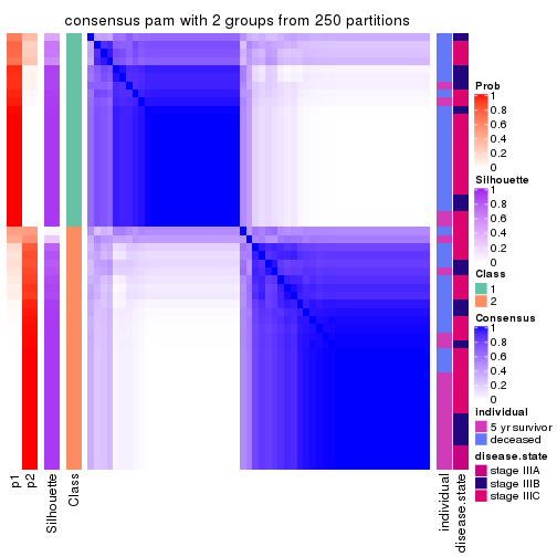
consensus_heatmap(res, k = 3)
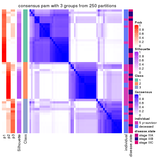
consensus_heatmap(res, k = 4)
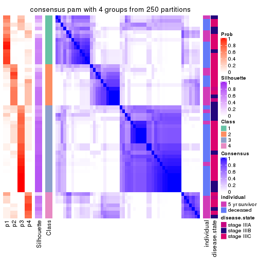
consensus_heatmap(res, k = 5)
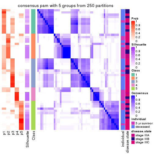
consensus_heatmap(res, k = 6)
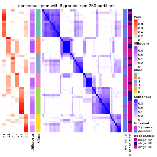
Heatmaps for the membership of samples in all partitions to see how consistent they are:
membership_heatmap(res, k = 2)
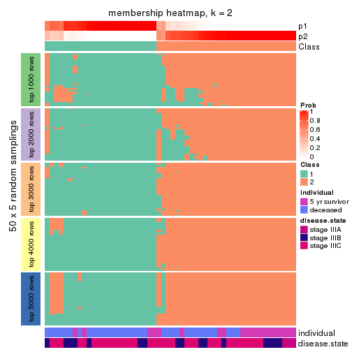
membership_heatmap(res, k = 3)
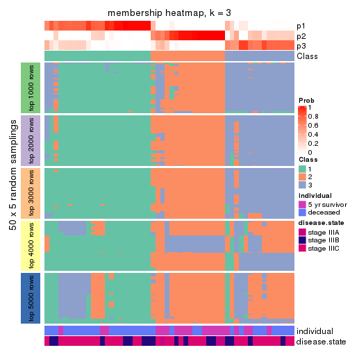
membership_heatmap(res, k = 4)
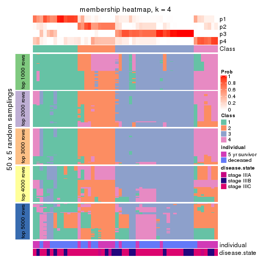
membership_heatmap(res, k = 5)
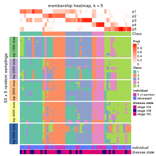
membership_heatmap(res, k = 6)
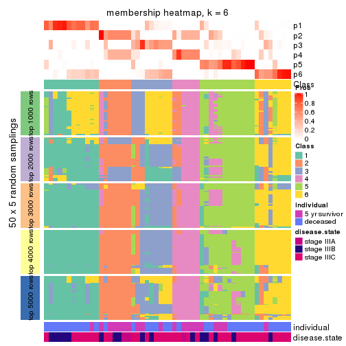
As soon as we have had the classes for columns, we can look for signatures which are significantly different between classes which can be candidate marks for certain classes. Following are the heatmaps for signatures.
Signature heatmaps where rows are scaled:
get_signatures(res, k = 2)
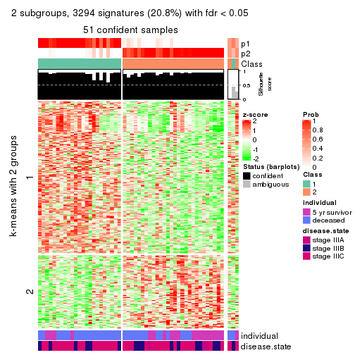
get_signatures(res, k = 3)
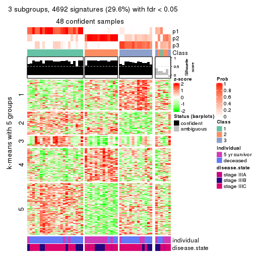
get_signatures(res, k = 4)
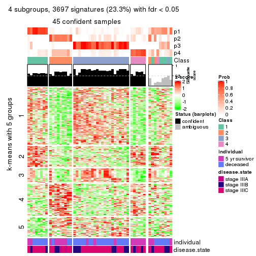
get_signatures(res, k = 5)
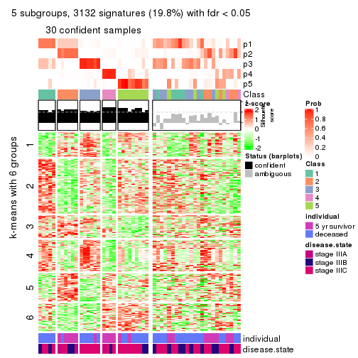
get_signatures(res, k = 6)
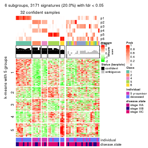
Signature heatmaps where rows are not scaled:
get_signatures(res, k = 2, scale_rows = FALSE)
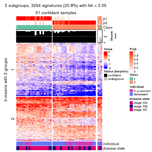
get_signatures(res, k = 3, scale_rows = FALSE)
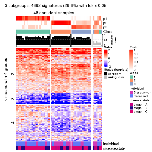
get_signatures(res, k = 4, scale_rows = FALSE)
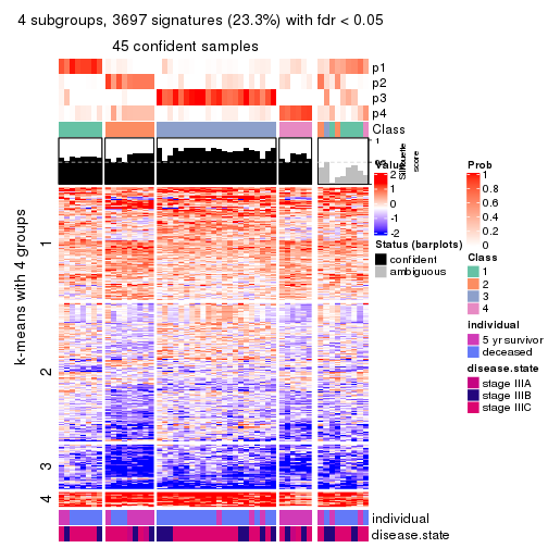
get_signatures(res, k = 5, scale_rows = FALSE)
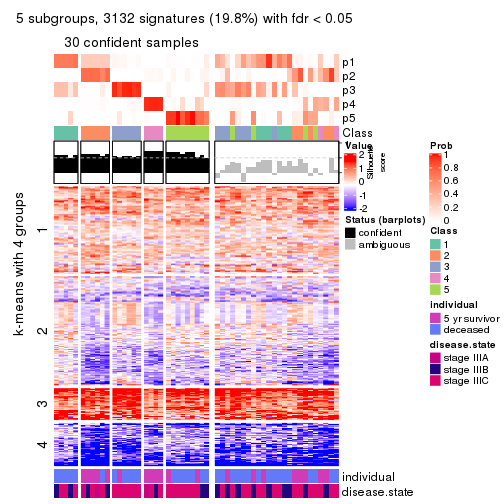
get_signatures(res, k = 6, scale_rows = FALSE)
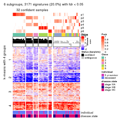
Compare the overlap of signatures from different k:
compare_signatures(res)
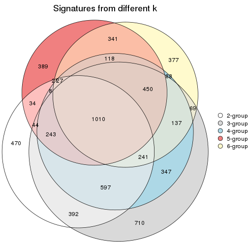
get_signature() returns a data frame invisibly. TO get the list of signatures, the function
call should be assigned to a variable explicitly. In following code, if plot argument is set
to FALSE, no heatmap is plotted while only the differential analysis is performed.
# code only for demonstration
tb = get_signature(res, k = ..., plot = FALSE)
An example of the output of tb is:
#> which_row fdr mean_1 mean_2 scaled_mean_1 scaled_mean_2 km
#> 1 38 0.042760348 8.373488 9.131774 -0.5533452 0.5164555 1
#> 2 40 0.018707592 7.106213 8.469186 -0.6173731 0.5762149 1
#> 3 55 0.019134737 10.221463 11.207825 -0.6159697 0.5749050 1
#> 4 59 0.006059896 5.921854 7.869574 -0.6899429 0.6439467 1
#> 5 60 0.018055526 8.928898 10.211722 -0.6204761 0.5791110 1
#> 6 98 0.009384629 15.714769 14.887706 0.6635654 -0.6193277 2
...
The columns in tb are:
which_row: row indices corresponding to the input matrix.fdr: FDR for the differential test. mean_x: The mean value in group x.scaled_mean_x: The mean value in group x after rows are scaled.km: Row groups if k-means clustering is applied to rows.UMAP plot which shows how samples are separated.
dimension_reduction(res, k = 2, method = "UMAP")
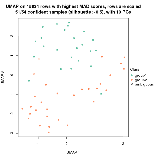
dimension_reduction(res, k = 3, method = "UMAP")
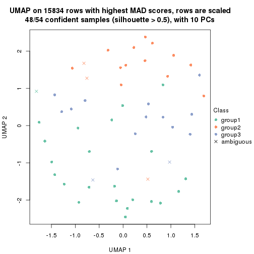
dimension_reduction(res, k = 4, method = "UMAP")
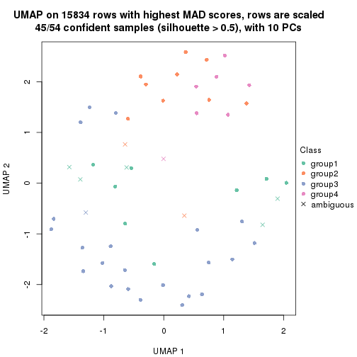
dimension_reduction(res, k = 5, method = "UMAP")
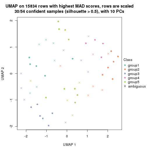
dimension_reduction(res, k = 6, method = "UMAP")
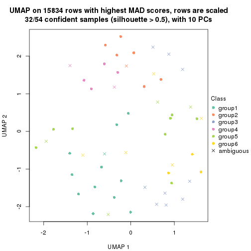
Following heatmap shows how subgroups are split when increasing k:
collect_classes(res)
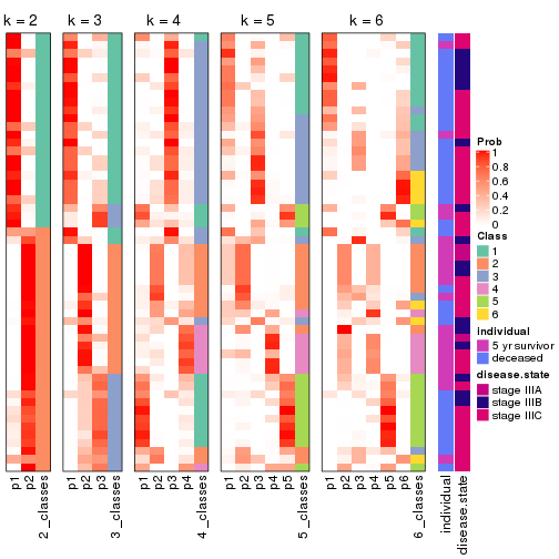
Test correlation between subgroups and known annotations. If the known annotation is numeric, one-way ANOVA test is applied, and if the known annotation is discrete, chi-squared contingency table test is applied.
test_to_known_factors(res)
#> n individual(p) disease.state(p) k
#> MAD:pam 51 0.017877 0.205 2
#> MAD:pam 48 0.000416 0.188 3
#> MAD:pam 45 0.000262 0.326 4
#> MAD:pam 30 0.002338 0.214 5
#> MAD:pam 32 0.001145 0.202 6
If matrix rows can be associated to genes, consider to use functional_enrichment(res,
...) to perform function enrichment for the signature genes. See this vignette for more detailed explanations.
The object with results only for a single top-value method and a single partition method can be extracted as:
res = res_list["MAD", "mclust"]
# you can also extract it by
# res = res_list["MAD:mclust"]
A summary of res and all the functions that can be applied to it:
res
#> A 'ConsensusPartition' object with k = 2, 3, 4, 5, 6.
#> On a matrix with 15834 rows and 54 columns.
#> Top rows (1000, 2000, 3000, 4000, 5000) are extracted by 'MAD' method.
#> Subgroups are detected by 'mclust' method.
#> Performed in total 1250 partitions by row resampling.
#> Best k for subgroups seems to be 5.
#>
#> Following methods can be applied to this 'ConsensusPartition' object:
#> [1] "cola_report" "collect_classes" "collect_plots"
#> [4] "collect_stats" "colnames" "compare_signatures"
#> [7] "consensus_heatmap" "dimension_reduction" "functional_enrichment"
#> [10] "get_anno_col" "get_anno" "get_classes"
#> [13] "get_consensus" "get_matrix" "get_membership"
#> [16] "get_param" "get_signatures" "get_stats"
#> [19] "is_best_k" "is_stable_k" "membership_heatmap"
#> [22] "ncol" "nrow" "plot_ecdf"
#> [25] "rownames" "select_partition_number" "show"
#> [28] "suggest_best_k" "test_to_known_factors"
collect_plots() function collects all the plots made from res for all k (number of partitions)
into one single page to provide an easy and fast comparison between different k.
collect_plots(res)
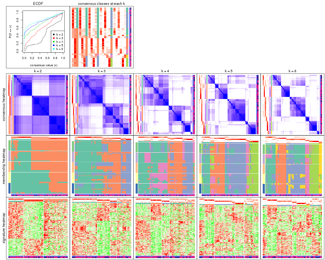
The plots are:
k and the heatmap of
predicted classes for each k.k.k.k.All the plots in panels can be made by individual functions and they are plotted later in this section.
select_partition_number() produces several plots showing different
statistics for choosing “optimized” k. There are following statistics:
k;k, the area increased is defined as \(A_k - A_{k-1}\).The detailed explanations of these statistics can be found in the cola vignette.
Generally speaking, lower PAC score, higher mean silhouette score or higher
concordance corresponds to better partition. Rand index and Jaccard index
measure how similar the current partition is compared to partition with k-1.
If they are too similar, we won't accept k is better than k-1.
select_partition_number(res)
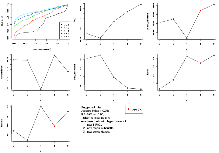
The numeric values for all these statistics can be obtained by get_stats().
get_stats(res)
#> k 1-PAC mean_silhouette concordance area_increased Rand Jaccard
#> 2 2 0.405 0.555 0.790 0.4154 0.535 0.535
#> 3 3 0.362 0.574 0.789 0.4536 0.644 0.434
#> 4 4 0.525 0.469 0.730 0.1935 0.922 0.805
#> 5 5 0.620 0.621 0.799 0.0633 0.843 0.586
#> 6 6 0.692 0.657 0.765 0.0513 0.936 0.747
suggest_best_k() suggests the best \(k\) based on these statistics. The rules are as follows:
suggest_best_k(res)
#> [1] 5
Following shows the table of the partitions (You need to click the show/hide
code output link to see it). The membership matrix (columns with name p*)
is inferred by
clue::cl_consensus()
function with the SE method. Basically the value in the membership matrix
represents the probability to belong to a certain group. The finall class
label for an item is determined with the group with highest probability it
belongs to.
In get_classes() function, the entropy is calculated from the membership
matrix and the silhouette score is calculated from the consensus matrix.
cbind(get_classes(res, k = 2), get_membership(res, k = 2))
#> class entropy silhouette p1 p2
#> GSM311939 2 0.2423 0.6385 0.040 0.960
#> GSM311963 2 0.1414 0.6478 0.020 0.980
#> GSM311973 2 0.3879 0.6382 0.076 0.924
#> GSM311940 2 0.2423 0.6385 0.040 0.960
#> GSM311953 2 0.0000 0.6437 0.000 1.000
#> GSM311974 2 0.0672 0.6481 0.008 0.992
#> GSM311975 1 0.9460 0.2471 0.636 0.364
#> GSM311977 2 0.1843 0.6452 0.028 0.972
#> GSM311982 2 0.9850 0.4303 0.428 0.572
#> GSM311990 2 0.0672 0.6481 0.008 0.992
#> GSM311943 1 0.2236 0.7919 0.964 0.036
#> GSM311944 2 0.9850 0.4303 0.428 0.572
#> GSM311946 2 0.2423 0.6504 0.040 0.960
#> GSM311956 2 0.0672 0.6481 0.008 0.992
#> GSM311967 2 0.2423 0.6472 0.040 0.960
#> GSM311968 2 0.9732 0.4544 0.404 0.596
#> GSM311972 1 0.3584 0.7782 0.932 0.068
#> GSM311980 2 0.0672 0.6481 0.008 0.992
#> GSM311981 2 0.9922 0.4144 0.448 0.552
#> GSM311988 2 0.2423 0.6385 0.040 0.960
#> GSM311957 2 0.9922 0.4144 0.448 0.552
#> GSM311960 2 0.9833 0.4358 0.424 0.576
#> GSM311971 2 0.9922 0.4144 0.448 0.552
#> GSM311976 1 0.9970 -0.1855 0.532 0.468
#> GSM311978 1 0.9323 0.2980 0.652 0.348
#> GSM311979 2 0.9922 0.4144 0.448 0.552
#> GSM311983 1 0.0938 0.7823 0.988 0.012
#> GSM311986 2 0.9922 0.4144 0.448 0.552
#> GSM311991 1 0.9286 0.3441 0.656 0.344
#> GSM311938 2 0.3431 0.6455 0.064 0.936
#> GSM311941 1 0.4298 0.7648 0.912 0.088
#> GSM311942 2 0.9896 0.4235 0.440 0.560
#> GSM311945 2 0.9896 0.4235 0.440 0.560
#> GSM311947 2 0.1184 0.6497 0.016 0.984
#> GSM311948 2 0.6712 0.5969 0.176 0.824
#> GSM311949 2 1.0000 0.3178 0.496 0.504
#> GSM311950 2 0.2423 0.6472 0.040 0.960
#> GSM311951 2 0.9850 0.4303 0.428 0.572
#> GSM311952 1 0.2236 0.7919 0.964 0.036
#> GSM311954 1 0.9833 -0.0438 0.576 0.424
#> GSM311955 1 0.2236 0.7919 0.964 0.036
#> GSM311958 1 0.2043 0.7904 0.968 0.032
#> GSM311959 1 0.8267 0.5446 0.740 0.260
#> GSM311961 1 0.0938 0.7823 0.988 0.012
#> GSM311962 1 0.0938 0.7823 0.988 0.012
#> GSM311964 2 0.9933 0.4049 0.452 0.548
#> GSM311965 2 0.9866 0.4287 0.432 0.568
#> GSM311966 1 0.0938 0.7823 0.988 0.012
#> GSM311969 1 0.2236 0.7919 0.964 0.036
#> GSM311970 2 0.1414 0.6478 0.020 0.980
#> GSM311984 1 0.5842 0.7027 0.860 0.140
#> GSM311985 1 0.2043 0.7904 0.968 0.032
#> GSM311987 2 0.9909 0.4207 0.444 0.556
#> GSM311989 2 0.9896 0.4235 0.440 0.560
cbind(get_classes(res, k = 3), get_membership(res, k = 3))
#> class entropy silhouette p1 p2 p3
#> GSM311939 2 0.0661 0.6375 0.008 0.988 0.004
#> GSM311963 2 0.1999 0.6474 0.012 0.952 0.036
#> GSM311973 2 0.5529 0.5073 0.000 0.704 0.296
#> GSM311940 2 0.0424 0.6342 0.008 0.992 0.000
#> GSM311953 2 0.2845 0.6397 0.012 0.920 0.068
#> GSM311974 2 0.5431 0.5218 0.000 0.716 0.284
#> GSM311975 1 0.4423 0.7736 0.864 0.048 0.088
#> GSM311977 2 0.0661 0.6375 0.008 0.988 0.004
#> GSM311982 1 0.8793 0.4463 0.552 0.140 0.308
#> GSM311990 3 0.6483 0.0921 0.004 0.452 0.544
#> GSM311943 1 0.2772 0.7672 0.916 0.004 0.080
#> GSM311944 1 0.9282 0.3141 0.468 0.164 0.368
#> GSM311946 2 0.7002 0.4811 0.048 0.672 0.280
#> GSM311956 2 0.5465 0.5177 0.000 0.712 0.288
#> GSM311967 2 0.7013 0.2944 0.028 0.608 0.364
#> GSM311968 3 0.1289 0.6937 0.000 0.032 0.968
#> GSM311972 1 0.4045 0.7676 0.872 0.024 0.104
#> GSM311980 2 0.5529 0.5073 0.000 0.704 0.296
#> GSM311981 2 0.9941 0.1276 0.324 0.384 0.292
#> GSM311988 2 0.0424 0.6342 0.008 0.992 0.000
#> GSM311957 1 0.8866 0.5383 0.572 0.180 0.248
#> GSM311960 3 0.5291 0.4726 0.000 0.268 0.732
#> GSM311971 1 0.9887 -0.0168 0.408 0.288 0.304
#> GSM311976 1 0.7505 0.6495 0.696 0.160 0.144
#> GSM311978 1 0.7097 0.6839 0.724 0.128 0.148
#> GSM311979 1 0.7672 0.6491 0.684 0.156 0.160
#> GSM311983 1 0.0237 0.7765 0.996 0.004 0.000
#> GSM311986 2 0.9753 0.0877 0.228 0.400 0.372
#> GSM311991 1 0.5036 0.7582 0.832 0.120 0.048
#> GSM311938 2 0.6441 0.4966 0.028 0.696 0.276
#> GSM311941 1 0.6174 0.7291 0.768 0.064 0.168
#> GSM311942 3 0.1163 0.6951 0.000 0.028 0.972
#> GSM311945 3 0.5393 0.5275 0.148 0.044 0.808
#> GSM311947 3 0.6489 0.0797 0.004 0.456 0.540
#> GSM311948 3 0.6432 0.1431 0.004 0.428 0.568
#> GSM311949 1 0.7327 0.6633 0.708 0.160 0.132
#> GSM311950 2 0.0983 0.6412 0.004 0.980 0.016
#> GSM311951 3 0.1163 0.6951 0.000 0.028 0.972
#> GSM311952 1 0.0475 0.7765 0.992 0.004 0.004
#> GSM311954 1 0.7710 0.6548 0.680 0.176 0.144
#> GSM311955 1 0.1647 0.7758 0.960 0.004 0.036
#> GSM311958 1 0.0237 0.7765 0.996 0.004 0.000
#> GSM311959 1 0.3459 0.7627 0.892 0.012 0.096
#> GSM311961 1 0.0237 0.7765 0.996 0.004 0.000
#> GSM311962 1 0.0237 0.7765 0.996 0.004 0.000
#> GSM311964 1 0.7451 0.6646 0.700 0.144 0.156
#> GSM311965 3 0.1163 0.6951 0.000 0.028 0.972
#> GSM311966 1 0.1170 0.7799 0.976 0.008 0.016
#> GSM311969 1 0.3030 0.7647 0.904 0.004 0.092
#> GSM311970 2 0.3425 0.6358 0.004 0.884 0.112
#> GSM311984 1 0.2845 0.7734 0.920 0.012 0.068
#> GSM311985 1 0.0237 0.7762 0.996 0.004 0.000
#> GSM311987 2 0.9773 0.0192 0.372 0.396 0.232
#> GSM311989 3 0.1163 0.6951 0.000 0.028 0.972
cbind(get_classes(res, k = 4), get_membership(res, k = 4))
#> class entropy silhouette p1 p2 p3 p4
#> GSM311939 2 0.1474 0.6770 0.000 0.948 0.000 0.052
#> GSM311963 2 0.0000 0.7134 0.000 1.000 0.000 0.000
#> GSM311973 2 0.5376 0.3442 0.000 0.588 0.396 0.016
#> GSM311940 2 0.0000 0.7134 0.000 1.000 0.000 0.000
#> GSM311953 2 0.2060 0.7001 0.000 0.932 0.052 0.016
#> GSM311974 2 0.4748 0.5560 0.000 0.716 0.268 0.016
#> GSM311975 1 0.4933 0.2347 0.568 0.000 0.000 0.432
#> GSM311977 2 0.0000 0.7134 0.000 1.000 0.000 0.000
#> GSM311982 1 0.7842 0.2975 0.456 0.004 0.272 0.268
#> GSM311990 3 0.7896 -0.0581 0.000 0.292 0.356 0.352
#> GSM311943 1 0.3764 0.5547 0.784 0.000 0.000 0.216
#> GSM311944 1 0.7208 0.2301 0.548 0.096 0.336 0.020
#> GSM311946 2 0.3877 0.6404 0.000 0.840 0.048 0.112
#> GSM311956 2 0.5339 0.3700 0.000 0.600 0.384 0.016
#> GSM311967 4 0.6882 0.4152 0.084 0.388 0.008 0.520
#> GSM311968 3 0.0000 0.7559 0.000 0.000 1.000 0.000
#> GSM311972 1 0.4222 0.5373 0.728 0.000 0.000 0.272
#> GSM311980 2 0.5459 0.2515 0.000 0.552 0.432 0.016
#> GSM311981 4 0.6916 0.5168 0.280 0.148 0.000 0.572
#> GSM311988 2 0.0000 0.7134 0.000 1.000 0.000 0.000
#> GSM311957 1 0.7011 0.4069 0.640 0.032 0.216 0.112
#> GSM311960 3 0.4072 0.5216 0.000 0.252 0.748 0.000
#> GSM311971 1 0.8283 0.2773 0.420 0.048 0.136 0.396
#> GSM311976 1 0.6025 0.4395 0.668 0.096 0.000 0.236
#> GSM311978 1 0.4456 0.5316 0.716 0.004 0.000 0.280
#> GSM311979 1 0.7291 0.4064 0.536 0.004 0.160 0.300
#> GSM311983 1 0.0188 0.6011 0.996 0.000 0.000 0.004
#> GSM311986 1 0.7002 0.0386 0.492 0.120 0.000 0.388
#> GSM311991 1 0.5685 -0.1569 0.516 0.024 0.000 0.460
#> GSM311938 2 0.6595 -0.0832 0.160 0.628 0.000 0.212
#> GSM311941 1 0.3975 0.5531 0.760 0.000 0.000 0.240
#> GSM311942 3 0.0000 0.7559 0.000 0.000 1.000 0.000
#> GSM311945 3 0.0000 0.7559 0.000 0.000 1.000 0.000
#> GSM311947 3 0.7896 -0.0581 0.000 0.292 0.356 0.352
#> GSM311948 3 0.4477 0.4190 0.000 0.312 0.688 0.000
#> GSM311949 1 0.4973 0.4740 0.644 0.008 0.000 0.348
#> GSM311950 2 0.3569 0.5016 0.000 0.804 0.000 0.196
#> GSM311951 3 0.0000 0.7559 0.000 0.000 1.000 0.000
#> GSM311952 1 0.1940 0.5994 0.924 0.000 0.000 0.076
#> GSM311954 1 0.4790 0.3069 0.620 0.000 0.000 0.380
#> GSM311955 1 0.3528 0.5472 0.808 0.000 0.000 0.192
#> GSM311958 1 0.3074 0.5675 0.848 0.000 0.000 0.152
#> GSM311959 1 0.4817 0.2924 0.612 0.000 0.000 0.388
#> GSM311961 1 0.0188 0.6012 0.996 0.000 0.000 0.004
#> GSM311962 1 0.0000 0.6009 1.000 0.000 0.000 0.000
#> GSM311964 1 0.6223 0.4226 0.552 0.004 0.048 0.396
#> GSM311965 3 0.0000 0.7559 0.000 0.000 1.000 0.000
#> GSM311966 1 0.3444 0.5656 0.816 0.000 0.000 0.184
#> GSM311969 1 0.3486 0.5497 0.812 0.000 0.000 0.188
#> GSM311970 2 0.0000 0.7134 0.000 1.000 0.000 0.000
#> GSM311984 1 0.3486 0.5497 0.812 0.000 0.000 0.188
#> GSM311985 1 0.0921 0.6004 0.972 0.000 0.000 0.028
#> GSM311987 1 0.7273 -0.1084 0.452 0.148 0.000 0.400
#> GSM311989 3 0.0000 0.7559 0.000 0.000 1.000 0.000
cbind(get_classes(res, k = 5), get_membership(res, k = 5))
#> class entropy silhouette p1 p2 p3 p4 p5
#> GSM311939 2 0.0566 0.698 0.004 0.984 0.000 0.012 0.000
#> GSM311963 2 0.0000 0.704 0.000 1.000 0.000 0.000 0.000
#> GSM311973 2 0.7771 0.279 0.056 0.340 0.000 0.288 0.316
#> GSM311940 2 0.0000 0.704 0.000 1.000 0.000 0.000 0.000
#> GSM311953 2 0.2806 0.673 0.000 0.844 0.000 0.152 0.004
#> GSM311974 2 0.6992 0.487 0.056 0.552 0.000 0.172 0.220
#> GSM311975 3 0.2723 0.740 0.124 0.000 0.864 0.012 0.000
#> GSM311977 2 0.0000 0.704 0.000 1.000 0.000 0.000 0.000
#> GSM311982 1 0.5491 0.369 0.580 0.000 0.056 0.008 0.356
#> GSM311990 4 0.4183 0.701 0.000 0.008 0.000 0.668 0.324
#> GSM311943 3 0.0898 0.787 0.020 0.000 0.972 0.008 0.000
#> GSM311944 5 0.4440 0.209 0.012 0.000 0.324 0.004 0.660
#> GSM311946 2 0.3272 0.658 0.120 0.848 0.000 0.016 0.016
#> GSM311956 2 0.7767 0.283 0.056 0.344 0.000 0.284 0.316
#> GSM311967 4 0.5379 0.510 0.004 0.124 0.164 0.700 0.008
#> GSM311968 5 0.1043 0.823 0.040 0.000 0.000 0.000 0.960
#> GSM311972 3 0.4452 -0.247 0.496 0.000 0.500 0.004 0.000
#> GSM311980 2 0.7774 0.253 0.056 0.328 0.000 0.288 0.328
#> GSM311981 3 0.6168 0.426 0.200 0.008 0.592 0.200 0.000
#> GSM311988 2 0.0000 0.704 0.000 1.000 0.000 0.000 0.000
#> GSM311957 1 0.6439 0.314 0.420 0.000 0.404 0.000 0.176
#> GSM311960 5 0.2732 0.691 0.000 0.000 0.000 0.160 0.840
#> GSM311971 1 0.3047 0.635 0.884 0.020 0.056 0.004 0.036
#> GSM311976 1 0.4297 0.219 0.528 0.000 0.472 0.000 0.000
#> GSM311978 1 0.3585 0.705 0.772 0.000 0.220 0.004 0.004
#> GSM311979 1 0.3983 0.672 0.812 0.000 0.088 0.008 0.092
#> GSM311983 3 0.2020 0.745 0.100 0.000 0.900 0.000 0.000
#> GSM311986 3 0.4113 0.684 0.076 0.000 0.784 0.140 0.000
#> GSM311991 3 0.5542 0.357 0.396 0.000 0.532 0.072 0.000
#> GSM311938 2 0.6664 0.391 0.172 0.628 0.128 0.064 0.008
#> GSM311941 3 0.0727 0.787 0.012 0.000 0.980 0.004 0.004
#> GSM311942 5 0.0000 0.848 0.000 0.000 0.000 0.000 1.000
#> GSM311945 5 0.0000 0.848 0.000 0.000 0.000 0.000 1.000
#> GSM311947 4 0.4066 0.701 0.000 0.004 0.000 0.672 0.324
#> GSM311948 5 0.3520 0.696 0.076 0.080 0.000 0.004 0.840
#> GSM311949 1 0.3534 0.672 0.744 0.000 0.256 0.000 0.000
#> GSM311950 2 0.3109 0.560 0.000 0.800 0.000 0.200 0.000
#> GSM311951 5 0.0000 0.848 0.000 0.000 0.000 0.000 1.000
#> GSM311952 3 0.1502 0.775 0.056 0.000 0.940 0.004 0.000
#> GSM311954 3 0.2813 0.742 0.108 0.000 0.868 0.024 0.000
#> GSM311955 3 0.0000 0.788 0.000 0.000 1.000 0.000 0.000
#> GSM311958 3 0.0324 0.788 0.004 0.000 0.992 0.004 0.000
#> GSM311959 3 0.2522 0.747 0.108 0.000 0.880 0.012 0.000
#> GSM311961 3 0.2516 0.722 0.140 0.000 0.860 0.000 0.000
#> GSM311962 3 0.2230 0.731 0.116 0.000 0.884 0.000 0.000
#> GSM311964 1 0.4010 0.711 0.784 0.000 0.160 0.000 0.056
#> GSM311965 5 0.0000 0.848 0.000 0.000 0.000 0.000 1.000
#> GSM311966 3 0.3876 0.380 0.316 0.000 0.684 0.000 0.000
#> GSM311969 3 0.0807 0.788 0.012 0.000 0.976 0.012 0.000
#> GSM311970 2 0.2516 0.667 0.000 0.860 0.000 0.140 0.000
#> GSM311984 3 0.0609 0.786 0.020 0.000 0.980 0.000 0.000
#> GSM311985 3 0.2536 0.721 0.128 0.000 0.868 0.004 0.000
#> GSM311987 3 0.4657 0.648 0.108 0.000 0.740 0.152 0.000
#> GSM311989 5 0.0000 0.848 0.000 0.000 0.000 0.000 1.000
cbind(get_classes(res, k = 6), get_membership(res, k = 6))
#> class entropy silhouette p1 p2 p3 p4 p5 p6
#> GSM311939 2 0.0363 0.872 0.000 0.988 0.000 0.000 0.000 0.012
#> GSM311963 2 0.0000 0.874 0.000 1.000 0.000 0.000 0.000 0.000
#> GSM311973 4 0.2554 0.902 0.000 0.048 0.000 0.876 0.076 0.000
#> GSM311940 2 0.0000 0.874 0.000 1.000 0.000 0.000 0.000 0.000
#> GSM311953 2 0.1075 0.854 0.000 0.952 0.000 0.048 0.000 0.000
#> GSM311974 4 0.4325 0.689 0.000 0.244 0.000 0.692 0.064 0.000
#> GSM311975 3 0.3324 0.611 0.008 0.000 0.832 0.084 0.000 0.076
#> GSM311977 2 0.0000 0.874 0.000 1.000 0.000 0.000 0.000 0.000
#> GSM311982 1 0.3878 0.208 0.644 0.000 0.004 0.000 0.348 0.004
#> GSM311990 6 0.3101 0.809 0.000 0.000 0.000 0.000 0.244 0.756
#> GSM311943 3 0.3588 0.659 0.144 0.000 0.804 0.032 0.000 0.020
#> GSM311944 5 0.2433 0.765 0.044 0.000 0.072 0.000 0.884 0.000
#> GSM311946 2 0.2263 0.825 0.036 0.900 0.004 0.060 0.000 0.000
#> GSM311956 4 0.2554 0.902 0.000 0.048 0.000 0.876 0.076 0.000
#> GSM311967 6 0.2612 0.616 0.000 0.108 0.016 0.008 0.000 0.868
#> GSM311968 5 0.1556 0.847 0.000 0.000 0.000 0.080 0.920 0.000
#> GSM311972 1 0.5288 0.446 0.588 0.000 0.300 0.008 0.000 0.104
#> GSM311980 4 0.2554 0.902 0.000 0.048 0.000 0.876 0.076 0.000
#> GSM311981 3 0.5104 0.496 0.012 0.004 0.640 0.080 0.000 0.264
#> GSM311988 2 0.0000 0.874 0.000 1.000 0.000 0.000 0.000 0.000
#> GSM311957 1 0.6355 0.305 0.536 0.000 0.260 0.000 0.136 0.068
#> GSM311960 5 0.1610 0.841 0.000 0.000 0.000 0.084 0.916 0.000
#> GSM311971 1 0.2001 0.489 0.900 0.000 0.004 0.092 0.004 0.000
#> GSM311976 1 0.5612 0.360 0.516 0.004 0.340 0.000 0.000 0.140
#> GSM311978 1 0.1858 0.611 0.904 0.000 0.092 0.000 0.000 0.004
#> GSM311979 1 0.1226 0.555 0.952 0.000 0.004 0.000 0.040 0.004
#> GSM311983 3 0.4546 0.575 0.204 0.000 0.692 0.000 0.000 0.104
#> GSM311986 3 0.5148 0.410 0.016 0.000 0.636 0.092 0.000 0.256
#> GSM311991 3 0.5672 0.484 0.076 0.004 0.652 0.084 0.000 0.184
#> GSM311938 2 0.4364 0.698 0.008 0.780 0.096 0.076 0.000 0.040
#> GSM311941 3 0.4118 0.653 0.144 0.000 0.780 0.016 0.012 0.048
#> GSM311942 5 0.0000 0.900 0.000 0.000 0.000 0.000 1.000 0.000
#> GSM311945 5 0.0000 0.900 0.000 0.000 0.000 0.000 1.000 0.000
#> GSM311947 6 0.3101 0.809 0.000 0.000 0.000 0.000 0.244 0.756
#> GSM311948 5 0.4723 0.558 0.036 0.036 0.004 0.224 0.700 0.000
#> GSM311949 1 0.4944 0.501 0.644 0.000 0.224 0.000 0.000 0.132
#> GSM311950 2 0.2823 0.720 0.000 0.796 0.000 0.000 0.000 0.204
#> GSM311951 5 0.0000 0.900 0.000 0.000 0.000 0.000 1.000 0.000
#> GSM311952 3 0.4992 0.526 0.260 0.000 0.624 0.000 0.000 0.116
#> GSM311954 3 0.3377 0.572 0.008 0.000 0.828 0.084 0.000 0.080
#> GSM311955 3 0.2312 0.671 0.112 0.000 0.876 0.000 0.000 0.012
#> GSM311958 3 0.4579 0.642 0.116 0.000 0.744 0.032 0.000 0.108
#> GSM311959 3 0.2849 0.599 0.008 0.000 0.864 0.084 0.000 0.044
#> GSM311961 3 0.4791 0.541 0.244 0.000 0.652 0.000 0.000 0.104
#> GSM311962 3 0.4518 0.578 0.200 0.000 0.696 0.000 0.000 0.104
#> GSM311964 1 0.3955 0.610 0.804 0.000 0.064 0.000 0.076 0.056
#> GSM311965 5 0.0000 0.900 0.000 0.000 0.000 0.000 1.000 0.000
#> GSM311966 1 0.5316 0.210 0.480 0.000 0.416 0.000 0.000 0.104
#> GSM311969 3 0.3845 0.660 0.120 0.000 0.800 0.032 0.000 0.048
#> GSM311970 2 0.5144 0.281 0.000 0.560 0.000 0.340 0.000 0.100
#> GSM311984 3 0.3189 0.645 0.184 0.000 0.796 0.000 0.000 0.020
#> GSM311985 3 0.5012 0.596 0.172 0.000 0.692 0.028 0.000 0.108
#> GSM311987 3 0.5029 0.351 0.008 0.000 0.632 0.092 0.000 0.268
#> GSM311989 5 0.0000 0.900 0.000 0.000 0.000 0.000 1.000 0.000
Heatmaps for the consensus matrix. It visualizes the probability of two samples to be in a same group.
consensus_heatmap(res, k = 2)
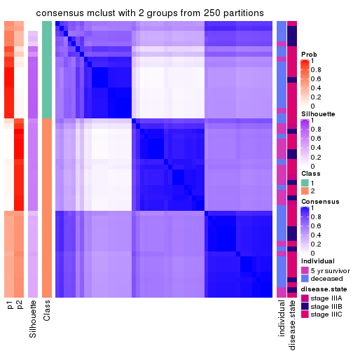
consensus_heatmap(res, k = 3)
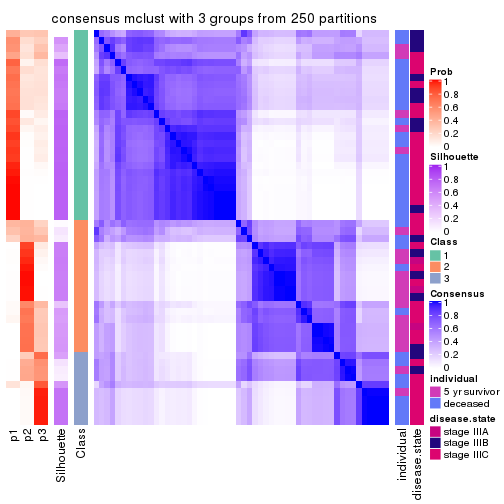
consensus_heatmap(res, k = 4)
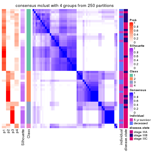
consensus_heatmap(res, k = 5)
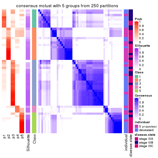
consensus_heatmap(res, k = 6)
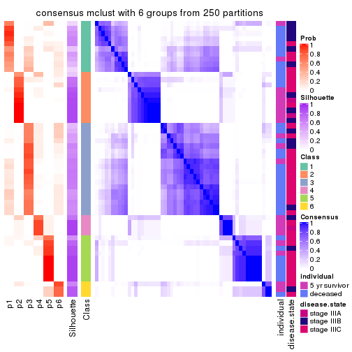
Heatmaps for the membership of samples in all partitions to see how consistent they are:
membership_heatmap(res, k = 2)
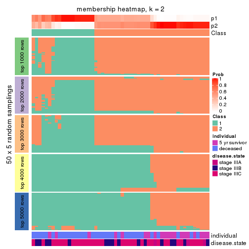
membership_heatmap(res, k = 3)
membership_heatmap(res, k = 4)
membership_heatmap(res, k = 5)
membership_heatmap(res, k = 6)
As soon as we have had the classes for columns, we can look for signatures which are significantly different between classes which can be candidate marks for certain classes. Following are the heatmaps for signatures.
Signature heatmaps where rows are scaled:
get_signatures(res, k = 2)
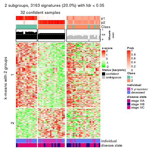
get_signatures(res, k = 3)
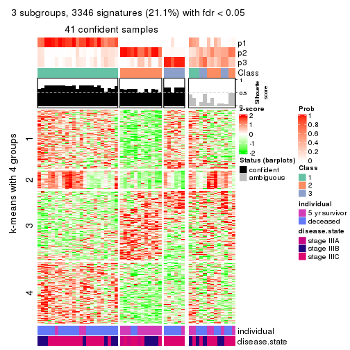
get_signatures(res, k = 4)
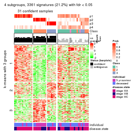
get_signatures(res, k = 5)
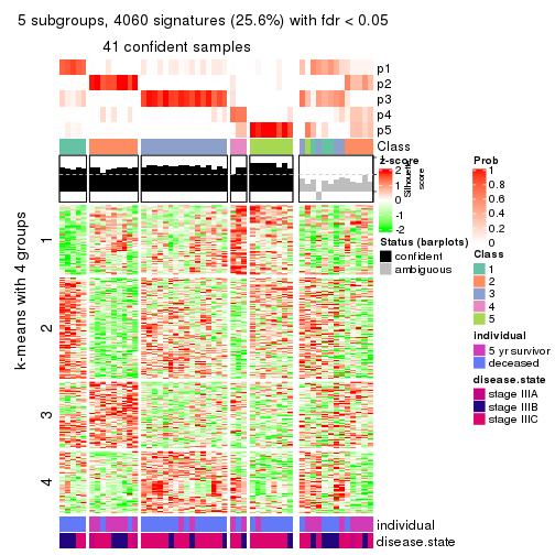
get_signatures(res, k = 6)
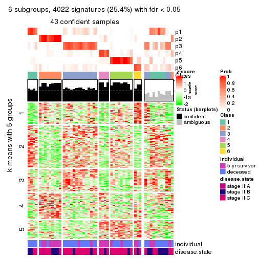
Signature heatmaps where rows are not scaled:
get_signatures(res, k = 2, scale_rows = FALSE)
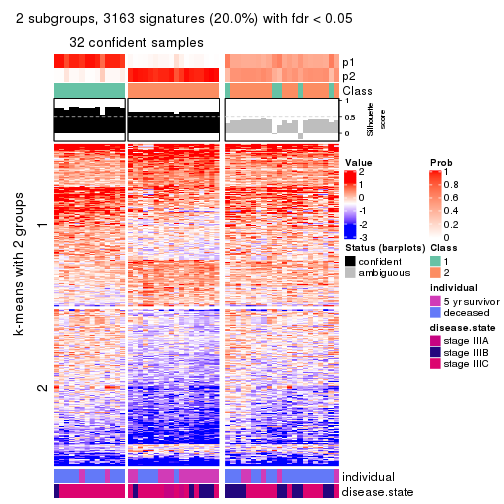
get_signatures(res, k = 3, scale_rows = FALSE)
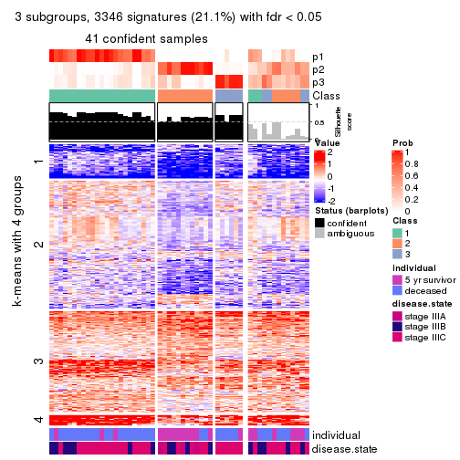
get_signatures(res, k = 4, scale_rows = FALSE)
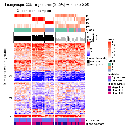
get_signatures(res, k = 5, scale_rows = FALSE)
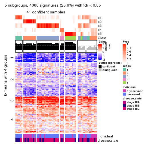
get_signatures(res, k = 6, scale_rows = FALSE)
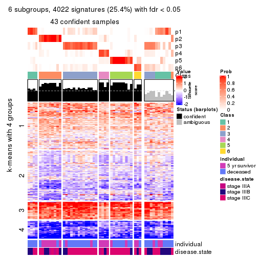
Compare the overlap of signatures from different k:
compare_signatures(res)
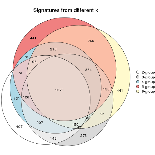
get_signature() returns a data frame invisibly. TO get the list of signatures, the function
call should be assigned to a variable explicitly. In following code, if plot argument is set
to FALSE, no heatmap is plotted while only the differential analysis is performed.
# code only for demonstration
tb = get_signature(res, k = ..., plot = FALSE)
An example of the output of tb is:
#> which_row fdr mean_1 mean_2 scaled_mean_1 scaled_mean_2 km
#> 1 38 0.042760348 8.373488 9.131774 -0.5533452 0.5164555 1
#> 2 40 0.018707592 7.106213 8.469186 -0.6173731 0.5762149 1
#> 3 55 0.019134737 10.221463 11.207825 -0.6159697 0.5749050 1
#> 4 59 0.006059896 5.921854 7.869574 -0.6899429 0.6439467 1
#> 5 60 0.018055526 8.928898 10.211722 -0.6204761 0.5791110 1
#> 6 98 0.009384629 15.714769 14.887706 0.6635654 -0.6193277 2
...
The columns in tb are:
which_row: row indices corresponding to the input matrix.fdr: FDR for the differential test. mean_x: The mean value in group x.scaled_mean_x: The mean value in group x after rows are scaled.km: Row groups if k-means clustering is applied to rows.UMAP plot which shows how samples are separated.
dimension_reduction(res, k = 2, method = "UMAP")
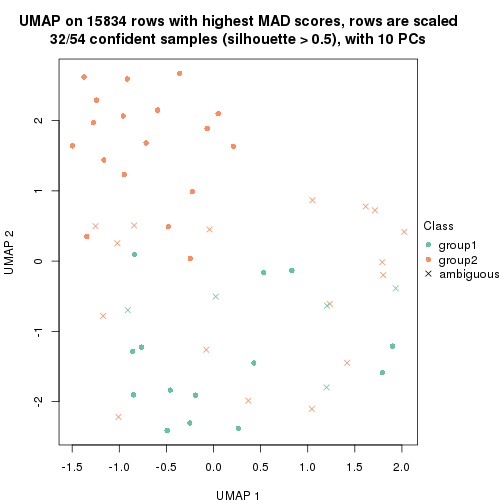
dimension_reduction(res, k = 3, method = "UMAP")
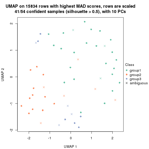
dimension_reduction(res, k = 4, method = "UMAP")
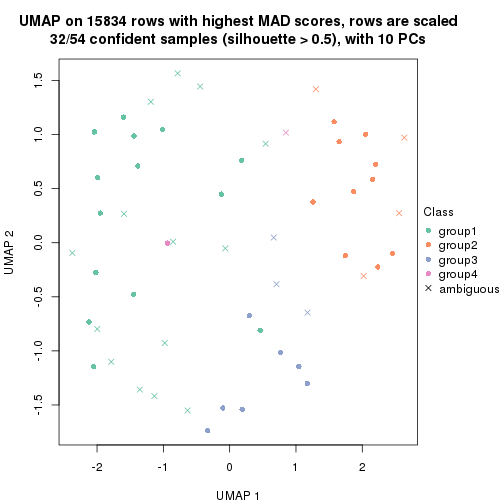
dimension_reduction(res, k = 5, method = "UMAP")
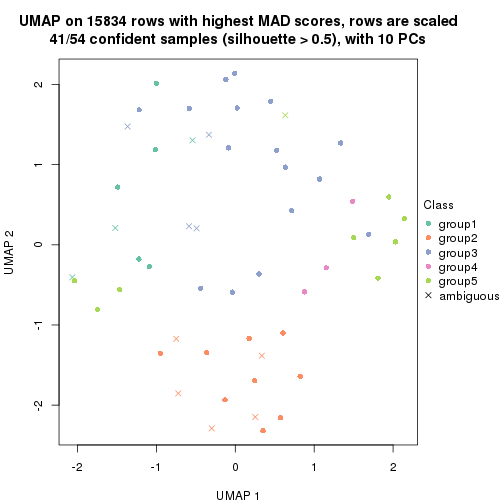
dimension_reduction(res, k = 6, method = "UMAP")
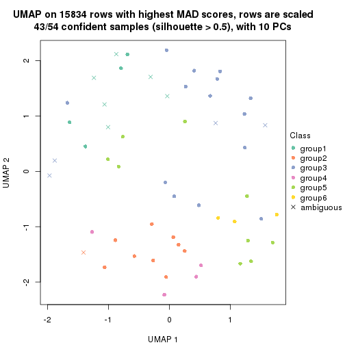
Following heatmap shows how subgroups are split when increasing k:
collect_classes(res)
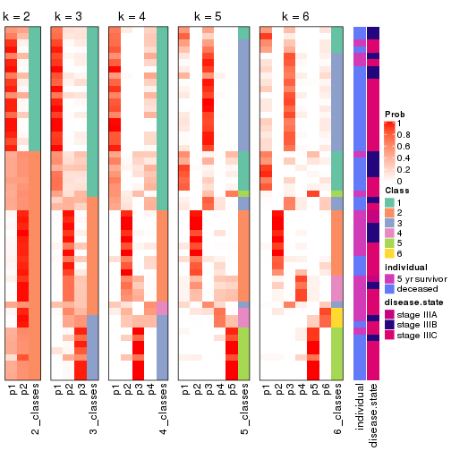
Test correlation between subgroups and known annotations. If the known annotation is numeric, one-way ANOVA test is applied, and if the known annotation is discrete, chi-squared contingency table test is applied.
test_to_known_factors(res)
#> n individual(p) disease.state(p) k
#> MAD:mclust 32 0.003720 0.0594 2
#> MAD:mclust 41 0.000107 0.0230 3
#> MAD:mclust 32 0.002643 0.1877 4
#> MAD:mclust 41 0.001487 0.1297 5
#> MAD:mclust 43 0.001236 0.2831 6
If matrix rows can be associated to genes, consider to use functional_enrichment(res,
...) to perform function enrichment for the signature genes. See this vignette for more detailed explanations.
The object with results only for a single top-value method and a single partition method can be extracted as:
res = res_list["MAD", "NMF"]
# you can also extract it by
# res = res_list["MAD:NMF"]
A summary of res and all the functions that can be applied to it:
res
#> A 'ConsensusPartition' object with k = 2, 3, 4, 5, 6.
#> On a matrix with 15834 rows and 54 columns.
#> Top rows (1000, 2000, 3000, 4000, 5000) are extracted by 'MAD' method.
#> Subgroups are detected by 'NMF' method.
#> Performed in total 1250 partitions by row resampling.
#> Best k for subgroups seems to be 2.
#>
#> Following methods can be applied to this 'ConsensusPartition' object:
#> [1] "cola_report" "collect_classes" "collect_plots"
#> [4] "collect_stats" "colnames" "compare_signatures"
#> [7] "consensus_heatmap" "dimension_reduction" "functional_enrichment"
#> [10] "get_anno_col" "get_anno" "get_classes"
#> [13] "get_consensus" "get_matrix" "get_membership"
#> [16] "get_param" "get_signatures" "get_stats"
#> [19] "is_best_k" "is_stable_k" "membership_heatmap"
#> [22] "ncol" "nrow" "plot_ecdf"
#> [25] "rownames" "select_partition_number" "show"
#> [28] "suggest_best_k" "test_to_known_factors"
collect_plots() function collects all the plots made from res for all k (number of partitions)
into one single page to provide an easy and fast comparison between different k.
collect_plots(res)
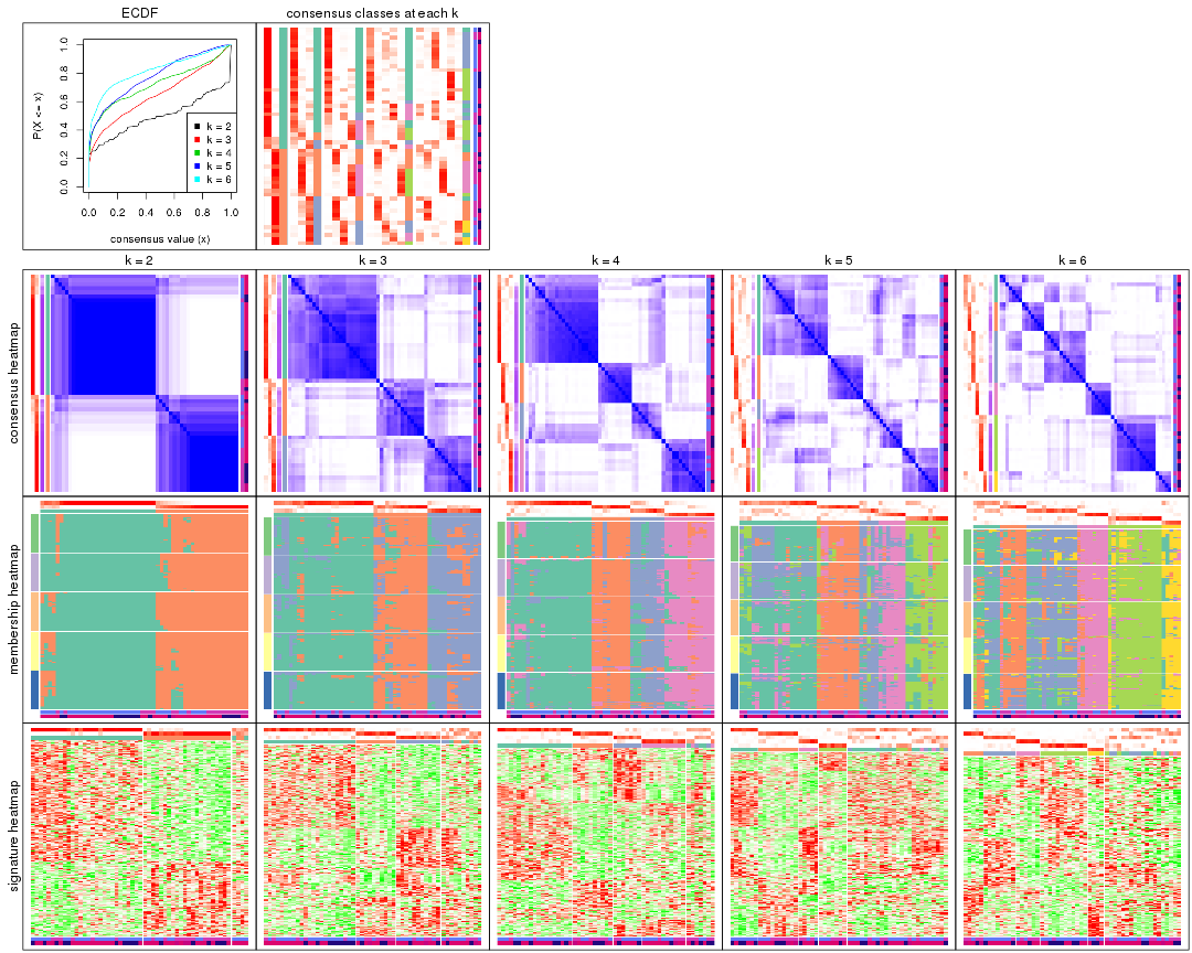
The plots are:
k and the heatmap of
predicted classes for each k.k.k.k.All the plots in panels can be made by individual functions and they are plotted later in this section.
select_partition_number() produces several plots showing different
statistics for choosing “optimized” k. There are following statistics:
k;k, the area increased is defined as \(A_k - A_{k-1}\).The detailed explanations of these statistics can be found in the cola vignette.
Generally speaking, lower PAC score, higher mean silhouette score or higher
concordance corresponds to better partition. Rand index and Jaccard index
measure how similar the current partition is compared to partition with k-1.
If they are too similar, we won't accept k is better than k-1.
select_partition_number(res)
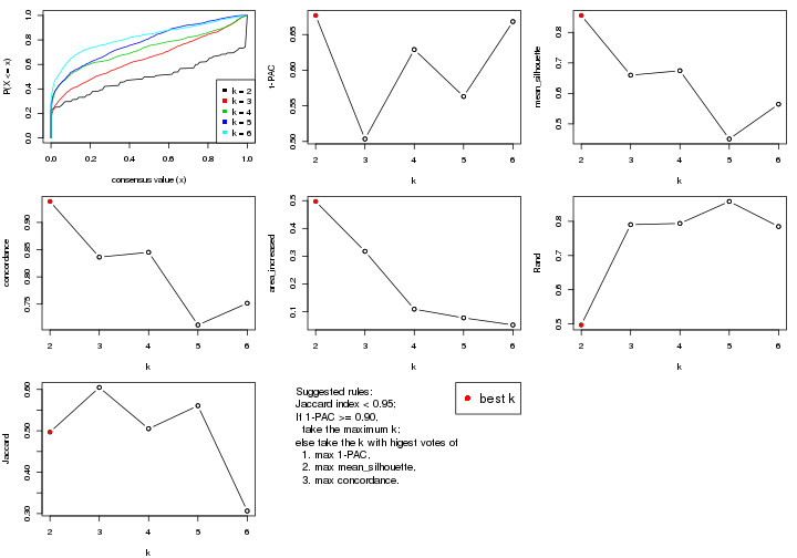
The numeric values for all these statistics can be obtained by get_stats().
get_stats(res)
#> k 1-PAC mean_silhouette concordance area_increased Rand Jaccard
#> 2 2 0.677 0.856 0.939 0.4970 0.497 0.497
#> 3 3 0.504 0.660 0.836 0.3174 0.790 0.605
#> 4 4 0.629 0.674 0.845 0.1090 0.794 0.505
#> 5 5 0.563 0.450 0.712 0.0777 0.858 0.561
#> 6 6 0.668 0.564 0.752 0.0521 0.785 0.306
suggest_best_k() suggests the best \(k\) based on these statistics. The rules are as follows:
suggest_best_k(res)
#> [1] 2
Following shows the table of the partitions (You need to click the show/hide
code output link to see it). The membership matrix (columns with name p*)
is inferred by
clue::cl_consensus()
function with the SE method. Basically the value in the membership matrix
represents the probability to belong to a certain group. The finall class
label for an item is determined with the group with highest probability it
belongs to.
In get_classes() function, the entropy is calculated from the membership
matrix and the silhouette score is calculated from the consensus matrix.
cbind(get_classes(res, k = 2), get_membership(res, k = 2))
#> class entropy silhouette p1 p2
#> GSM311939 2 0.0000 0.912 0.000 1.000
#> GSM311963 2 0.0000 0.912 0.000 1.000
#> GSM311973 2 0.6623 0.780 0.172 0.828
#> GSM311940 2 0.0000 0.912 0.000 1.000
#> GSM311953 2 0.0000 0.912 0.000 1.000
#> GSM311974 2 0.0000 0.912 0.000 1.000
#> GSM311975 1 0.0376 0.939 0.996 0.004
#> GSM311977 2 0.0000 0.912 0.000 1.000
#> GSM311982 1 0.0000 0.942 1.000 0.000
#> GSM311990 2 0.0000 0.912 0.000 1.000
#> GSM311943 1 0.0000 0.942 1.000 0.000
#> GSM311944 1 0.0000 0.942 1.000 0.000
#> GSM311946 2 0.0000 0.912 0.000 1.000
#> GSM311956 2 0.0000 0.912 0.000 1.000
#> GSM311967 2 0.0000 0.912 0.000 1.000
#> GSM311968 2 0.3274 0.884 0.060 0.940
#> GSM311972 1 0.0000 0.942 1.000 0.000
#> GSM311980 2 0.5629 0.824 0.132 0.868
#> GSM311981 1 0.8327 0.610 0.736 0.264
#> GSM311988 2 0.0000 0.912 0.000 1.000
#> GSM311957 1 0.0000 0.942 1.000 0.000
#> GSM311960 1 0.0000 0.942 1.000 0.000
#> GSM311971 1 0.0000 0.942 1.000 0.000
#> GSM311976 1 0.0000 0.942 1.000 0.000
#> GSM311978 1 0.0000 0.942 1.000 0.000
#> GSM311979 1 0.0000 0.942 1.000 0.000
#> GSM311983 1 0.0000 0.942 1.000 0.000
#> GSM311986 2 0.7299 0.743 0.204 0.796
#> GSM311991 1 0.2603 0.904 0.956 0.044
#> GSM311938 2 0.0000 0.912 0.000 1.000
#> GSM311941 1 0.7139 0.729 0.804 0.196
#> GSM311942 2 0.9970 0.145 0.468 0.532
#> GSM311945 1 0.0000 0.942 1.000 0.000
#> GSM311947 2 0.0000 0.912 0.000 1.000
#> GSM311948 2 0.3431 0.881 0.064 0.936
#> GSM311949 1 0.0000 0.942 1.000 0.000
#> GSM311950 2 0.0000 0.912 0.000 1.000
#> GSM311951 1 0.9286 0.440 0.656 0.344
#> GSM311952 1 0.0000 0.942 1.000 0.000
#> GSM311954 2 0.8443 0.638 0.272 0.728
#> GSM311955 1 0.0000 0.942 1.000 0.000
#> GSM311958 1 0.0000 0.942 1.000 0.000
#> GSM311959 1 0.8081 0.643 0.752 0.248
#> GSM311961 1 0.0000 0.942 1.000 0.000
#> GSM311962 1 0.0000 0.942 1.000 0.000
#> GSM311964 1 0.0000 0.942 1.000 0.000
#> GSM311965 2 0.9323 0.497 0.348 0.652
#> GSM311966 1 0.0000 0.942 1.000 0.000
#> GSM311969 1 0.0000 0.942 1.000 0.000
#> GSM311970 2 0.4815 0.848 0.104 0.896
#> GSM311984 1 0.9552 0.366 0.624 0.376
#> GSM311985 1 0.0000 0.942 1.000 0.000
#> GSM311987 2 0.1414 0.904 0.020 0.980
#> GSM311989 1 0.0000 0.942 1.000 0.000
cbind(get_classes(res, k = 3), get_membership(res, k = 3))
#> class entropy silhouette p1 p2 p3
#> GSM311939 3 0.5621 0.566234 0.000 0.308 0.692
#> GSM311963 3 0.6062 0.415750 0.000 0.384 0.616
#> GSM311973 2 0.0829 0.741810 0.012 0.984 0.004
#> GSM311940 3 0.5591 0.567187 0.000 0.304 0.696
#> GSM311953 2 0.3267 0.683365 0.000 0.884 0.116
#> GSM311974 2 0.1964 0.721807 0.000 0.944 0.056
#> GSM311975 1 0.5591 0.617860 0.696 0.000 0.304
#> GSM311977 2 0.6295 -0.121752 0.000 0.528 0.472
#> GSM311982 1 0.3816 0.770200 0.852 0.148 0.000
#> GSM311990 3 0.5882 0.445082 0.000 0.348 0.652
#> GSM311943 1 0.1411 0.844339 0.964 0.000 0.036
#> GSM311944 1 0.2625 0.819758 0.916 0.084 0.000
#> GSM311946 2 0.4702 0.578619 0.000 0.788 0.212
#> GSM311956 2 0.0747 0.738792 0.000 0.984 0.016
#> GSM311967 3 0.0892 0.736932 0.000 0.020 0.980
#> GSM311968 2 0.1453 0.740053 0.008 0.968 0.024
#> GSM311972 1 0.1031 0.841475 0.976 0.024 0.000
#> GSM311980 2 0.0592 0.741543 0.012 0.988 0.000
#> GSM311981 1 0.6625 0.337547 0.552 0.008 0.440
#> GSM311988 3 0.4555 0.673392 0.000 0.200 0.800
#> GSM311957 1 0.0892 0.842718 0.980 0.020 0.000
#> GSM311960 2 0.4796 0.601453 0.220 0.780 0.000
#> GSM311971 1 0.4733 0.728419 0.800 0.196 0.004
#> GSM311976 1 0.2165 0.837587 0.936 0.000 0.064
#> GSM311978 1 0.1964 0.830138 0.944 0.056 0.000
#> GSM311979 1 0.2261 0.825267 0.932 0.068 0.000
#> GSM311983 1 0.2066 0.837790 0.940 0.000 0.060
#> GSM311986 3 0.1860 0.729520 0.052 0.000 0.948
#> GSM311991 1 0.6297 0.522165 0.640 0.008 0.352
#> GSM311938 3 0.1964 0.738032 0.000 0.056 0.944
#> GSM311941 1 0.5968 0.429156 0.636 0.000 0.364
#> GSM311942 2 0.8550 0.430037 0.176 0.608 0.216
#> GSM311945 1 0.5968 0.427621 0.636 0.364 0.000
#> GSM311947 3 0.5465 0.509649 0.000 0.288 0.712
#> GSM311948 2 0.2229 0.740460 0.012 0.944 0.044
#> GSM311949 1 0.0661 0.845663 0.988 0.008 0.004
#> GSM311950 3 0.2537 0.729743 0.000 0.080 0.920
#> GSM311951 2 0.7665 -0.000705 0.456 0.500 0.044
#> GSM311952 1 0.1031 0.845079 0.976 0.000 0.024
#> GSM311954 3 0.2625 0.712410 0.084 0.000 0.916
#> GSM311955 1 0.5785 0.571639 0.668 0.000 0.332
#> GSM311958 1 0.2448 0.831604 0.924 0.000 0.076
#> GSM311959 3 0.4062 0.651442 0.164 0.000 0.836
#> GSM311961 1 0.1753 0.840992 0.952 0.000 0.048
#> GSM311962 1 0.1964 0.839943 0.944 0.000 0.056
#> GSM311964 1 0.2165 0.827383 0.936 0.064 0.000
#> GSM311965 2 0.4745 0.685646 0.080 0.852 0.068
#> GSM311966 1 0.0424 0.845756 0.992 0.000 0.008
#> GSM311969 1 0.4062 0.772919 0.836 0.000 0.164
#> GSM311970 2 0.5848 0.489168 0.012 0.720 0.268
#> GSM311984 3 0.5905 0.361948 0.352 0.000 0.648
#> GSM311985 1 0.0237 0.845224 0.996 0.000 0.004
#> GSM311987 3 0.1529 0.731837 0.040 0.000 0.960
#> GSM311989 1 0.4605 0.709268 0.796 0.204 0.000
cbind(get_classes(res, k = 4), get_membership(res, k = 4))
#> class entropy silhouette p1 p2 p3 p4
#> GSM311939 2 0.0657 0.8909 0.000 0.984 0.004 0.012
#> GSM311963 2 0.1004 0.8923 0.004 0.972 0.000 0.024
#> GSM311973 4 0.4770 0.5664 0.012 0.288 0.000 0.700
#> GSM311940 2 0.1833 0.8890 0.000 0.944 0.032 0.024
#> GSM311953 2 0.2408 0.8634 0.000 0.896 0.000 0.104
#> GSM311974 4 0.4699 0.4623 0.000 0.320 0.004 0.676
#> GSM311975 3 0.5313 0.2197 0.456 0.004 0.536 0.004
#> GSM311977 2 0.1211 0.8911 0.000 0.960 0.000 0.040
#> GSM311982 4 0.4955 0.1850 0.444 0.000 0.000 0.556
#> GSM311990 3 0.5429 0.5097 0.000 0.072 0.720 0.208
#> GSM311943 1 0.0895 0.8138 0.976 0.000 0.020 0.004
#> GSM311944 1 0.5295 -0.0104 0.504 0.000 0.008 0.488
#> GSM311946 2 0.2081 0.8746 0.000 0.916 0.000 0.084
#> GSM311956 4 0.2125 0.8003 0.000 0.076 0.004 0.920
#> GSM311967 3 0.0524 0.6272 0.000 0.004 0.988 0.008
#> GSM311968 4 0.0657 0.8165 0.000 0.004 0.012 0.984
#> GSM311972 1 0.1798 0.8018 0.944 0.000 0.040 0.016
#> GSM311980 4 0.2530 0.7827 0.000 0.112 0.000 0.888
#> GSM311981 3 0.5712 0.3329 0.408 0.016 0.568 0.008
#> GSM311988 2 0.0524 0.8819 0.004 0.988 0.008 0.000
#> GSM311957 1 0.1902 0.7868 0.932 0.004 0.000 0.064
#> GSM311960 4 0.1716 0.8180 0.064 0.000 0.000 0.936
#> GSM311971 1 0.6037 0.5639 0.688 0.156 0.000 0.156
#> GSM311976 1 0.1004 0.8126 0.972 0.024 0.004 0.000
#> GSM311978 1 0.0817 0.8084 0.976 0.000 0.000 0.024
#> GSM311979 1 0.3444 0.6840 0.816 0.000 0.000 0.184
#> GSM311983 1 0.0927 0.8123 0.976 0.008 0.016 0.000
#> GSM311986 3 0.4669 0.6230 0.100 0.092 0.804 0.004
#> GSM311991 1 0.6921 -0.2688 0.456 0.092 0.448 0.004
#> GSM311938 2 0.3680 0.7457 0.008 0.828 0.160 0.004
#> GSM311941 1 0.6081 0.1396 0.564 0.028 0.396 0.012
#> GSM311942 4 0.2010 0.8155 0.040 0.012 0.008 0.940
#> GSM311945 4 0.2469 0.7974 0.108 0.000 0.000 0.892
#> GSM311947 3 0.4088 0.5824 0.000 0.040 0.820 0.140
#> GSM311948 4 0.2021 0.8098 0.000 0.056 0.012 0.932
#> GSM311949 1 0.1545 0.8061 0.952 0.040 0.000 0.008
#> GSM311950 2 0.4677 0.5354 0.000 0.680 0.316 0.004
#> GSM311951 4 0.2334 0.8058 0.088 0.000 0.004 0.908
#> GSM311952 1 0.0336 0.8140 0.992 0.000 0.008 0.000
#> GSM311954 3 0.6179 0.5095 0.320 0.072 0.608 0.000
#> GSM311955 1 0.2805 0.7575 0.888 0.012 0.100 0.000
#> GSM311958 1 0.1902 0.7979 0.932 0.000 0.064 0.004
#> GSM311959 3 0.4832 0.5230 0.312 0.004 0.680 0.004
#> GSM311961 1 0.1443 0.8086 0.960 0.008 0.028 0.004
#> GSM311962 1 0.0927 0.8123 0.976 0.008 0.016 0.000
#> GSM311964 1 0.3791 0.6646 0.796 0.000 0.004 0.200
#> GSM311965 4 0.0844 0.8173 0.004 0.004 0.012 0.980
#> GSM311966 1 0.0188 0.8137 0.996 0.004 0.000 0.000
#> GSM311969 1 0.2981 0.7558 0.888 0.016 0.092 0.004
#> GSM311970 2 0.4030 0.8411 0.000 0.836 0.092 0.072
#> GSM311984 1 0.5540 0.5653 0.740 0.148 0.108 0.004
#> GSM311985 1 0.0376 0.8131 0.992 0.000 0.004 0.004
#> GSM311987 3 0.2457 0.6186 0.008 0.076 0.912 0.004
#> GSM311989 4 0.3311 0.7363 0.172 0.000 0.000 0.828
cbind(get_classes(res, k = 5), get_membership(res, k = 5))
#> class entropy silhouette p1 p2 p3 p4 p5
#> GSM311939 2 0.2233 0.7758 0.004 0.892 0.104 0.000 0.000
#> GSM311963 2 0.1043 0.7925 0.000 0.960 0.040 0.000 0.000
#> GSM311973 2 0.4848 0.2378 0.024 0.556 0.000 0.000 0.420
#> GSM311940 2 0.2349 0.7724 0.000 0.900 0.004 0.084 0.012
#> GSM311953 2 0.2628 0.7731 0.000 0.884 0.028 0.000 0.088
#> GSM311974 5 0.3300 0.5241 0.000 0.204 0.004 0.000 0.792
#> GSM311975 4 0.4054 0.5727 0.028 0.000 0.224 0.748 0.000
#> GSM311977 2 0.1329 0.7867 0.000 0.956 0.004 0.032 0.008
#> GSM311982 1 0.3274 0.4416 0.780 0.000 0.000 0.000 0.220
#> GSM311990 3 0.5708 -0.0318 0.000 0.000 0.556 0.096 0.348
#> GSM311943 1 0.4921 0.3606 0.604 0.000 0.360 0.036 0.000
#> GSM311944 1 0.6832 0.3091 0.524 0.000 0.160 0.032 0.284
#> GSM311946 2 0.3273 0.7673 0.004 0.848 0.112 0.000 0.036
#> GSM311956 5 0.2052 0.6507 0.000 0.080 0.004 0.004 0.912
#> GSM311967 4 0.3558 0.5980 0.000 0.000 0.108 0.828 0.064
#> GSM311968 5 0.1018 0.6604 0.016 0.000 0.016 0.000 0.968
#> GSM311972 1 0.4882 0.0934 0.540 0.000 0.012 0.440 0.008
#> GSM311980 5 0.3516 0.6041 0.020 0.164 0.004 0.000 0.812
#> GSM311981 4 0.0324 0.6790 0.004 0.000 0.000 0.992 0.004
#> GSM311988 2 0.2583 0.7601 0.004 0.864 0.132 0.000 0.000
#> GSM311957 1 0.2011 0.5794 0.928 0.020 0.044 0.000 0.008
#> GSM311960 5 0.4201 0.4457 0.408 0.000 0.000 0.000 0.592
#> GSM311971 1 0.3517 0.5398 0.832 0.100 0.000 0.000 0.068
#> GSM311976 1 0.5811 0.3554 0.596 0.140 0.000 0.264 0.000
#> GSM311978 1 0.0865 0.5836 0.972 0.000 0.000 0.004 0.024
#> GSM311979 1 0.1608 0.5708 0.928 0.000 0.000 0.000 0.072
#> GSM311983 1 0.5388 0.3333 0.580 0.004 0.360 0.056 0.000
#> GSM311986 3 0.2026 0.3254 0.016 0.044 0.928 0.012 0.000
#> GSM311991 4 0.1331 0.6937 0.008 0.000 0.040 0.952 0.000
#> GSM311938 2 0.3231 0.7015 0.004 0.800 0.196 0.000 0.000
#> GSM311941 1 0.5713 0.2623 0.604 0.000 0.316 0.024 0.056
#> GSM311942 5 0.4437 0.5100 0.316 0.000 0.020 0.000 0.664
#> GSM311945 5 0.4552 0.3189 0.468 0.000 0.008 0.000 0.524
#> GSM311947 5 0.6381 0.0150 0.000 0.000 0.364 0.172 0.464
#> GSM311948 5 0.1907 0.6423 0.000 0.044 0.028 0.000 0.928
#> GSM311949 1 0.1579 0.5852 0.944 0.032 0.000 0.024 0.000
#> GSM311950 2 0.4906 0.5585 0.000 0.640 0.028 0.324 0.008
#> GSM311951 5 0.4537 0.3907 0.396 0.000 0.012 0.000 0.592
#> GSM311952 1 0.5144 0.3498 0.604 0.016 0.356 0.024 0.000
#> GSM311954 4 0.5914 0.4426 0.040 0.068 0.260 0.632 0.000
#> GSM311955 1 0.6418 0.1174 0.420 0.000 0.408 0.172 0.000
#> GSM311958 4 0.6207 -0.0495 0.400 0.000 0.140 0.460 0.000
#> GSM311959 4 0.2850 0.6863 0.036 0.000 0.092 0.872 0.000
#> GSM311961 1 0.7503 0.1308 0.400 0.040 0.292 0.268 0.000
#> GSM311962 1 0.5637 0.3724 0.612 0.024 0.312 0.052 0.000
#> GSM311964 1 0.2448 0.5613 0.892 0.000 0.000 0.020 0.088
#> GSM311965 5 0.1106 0.6564 0.012 0.000 0.024 0.000 0.964
#> GSM311966 1 0.2804 0.5726 0.884 0.004 0.044 0.068 0.000
#> GSM311969 3 0.5507 -0.2860 0.456 0.000 0.480 0.064 0.000
#> GSM311970 2 0.4467 0.6627 0.000 0.724 0.012 0.240 0.024
#> GSM311984 3 0.6493 0.1124 0.292 0.196 0.508 0.004 0.000
#> GSM311985 1 0.4181 0.4631 0.712 0.000 0.020 0.268 0.000
#> GSM311987 3 0.4275 0.0487 0.000 0.008 0.696 0.288 0.008
#> GSM311989 1 0.5280 -0.0558 0.560 0.000 0.036 0.008 0.396
cbind(get_classes(res, k = 6), get_membership(res, k = 6))
#> class entropy silhouette p1 p2 p3 p4 p5 p6
#> GSM311939 2 0.0912 0.778 0.004 0.972 0.012 0.004 0.000 0.008
#> GSM311963 2 0.1371 0.773 0.040 0.948 0.004 0.004 0.000 0.004
#> GSM311973 4 0.5592 0.298 0.096 0.316 0.000 0.568 0.008 0.012
#> GSM311940 2 0.4329 0.455 0.404 0.576 0.000 0.008 0.000 0.012
#> GSM311953 4 0.4217 0.130 0.000 0.464 0.004 0.524 0.000 0.008
#> GSM311974 4 0.1204 0.805 0.000 0.056 0.000 0.944 0.000 0.000
#> GSM311975 3 0.3655 0.567 0.096 0.000 0.792 0.000 0.000 0.112
#> GSM311977 2 0.3604 0.668 0.216 0.760 0.000 0.012 0.000 0.012
#> GSM311982 5 0.2805 0.771 0.000 0.000 0.012 0.160 0.828 0.000
#> GSM311990 6 0.2100 0.699 0.000 0.004 0.000 0.112 0.000 0.884
#> GSM311943 3 0.4768 0.498 0.004 0.004 0.652 0.000 0.276 0.064
#> GSM311944 5 0.7347 0.189 0.000 0.000 0.140 0.212 0.400 0.248
#> GSM311946 2 0.4787 0.497 0.008 0.680 0.076 0.232 0.000 0.004
#> GSM311956 4 0.0436 0.815 0.000 0.004 0.000 0.988 0.004 0.004
#> GSM311967 6 0.4338 0.331 0.484 0.000 0.020 0.000 0.000 0.496
#> GSM311968 4 0.0520 0.811 0.000 0.000 0.000 0.984 0.008 0.008
#> GSM311972 3 0.4687 0.284 0.296 0.000 0.632 0.000 0.072 0.000
#> GSM311980 4 0.0982 0.812 0.004 0.020 0.000 0.968 0.004 0.004
#> GSM311981 1 0.4218 0.332 0.616 0.000 0.360 0.000 0.000 0.024
#> GSM311988 2 0.1065 0.777 0.000 0.964 0.008 0.008 0.000 0.020
#> GSM311957 5 0.0993 0.830 0.000 0.012 0.024 0.000 0.964 0.000
#> GSM311960 5 0.1327 0.827 0.000 0.000 0.000 0.064 0.936 0.000
#> GSM311971 5 0.0582 0.832 0.004 0.004 0.004 0.004 0.984 0.000
#> GSM311976 1 0.6500 0.102 0.444 0.052 0.148 0.000 0.356 0.000
#> GSM311978 5 0.1036 0.830 0.008 0.000 0.024 0.000 0.964 0.004
#> GSM311979 5 0.0260 0.832 0.000 0.000 0.008 0.000 0.992 0.000
#> GSM311983 3 0.3488 0.665 0.000 0.084 0.832 0.000 0.052 0.032
#> GSM311986 6 0.3110 0.653 0.004 0.052 0.092 0.000 0.004 0.848
#> GSM311991 1 0.4091 0.175 0.520 0.000 0.472 0.000 0.000 0.008
#> GSM311938 2 0.3402 0.707 0.056 0.844 0.068 0.004 0.000 0.028
#> GSM311941 5 0.5017 0.102 0.036 0.000 0.020 0.000 0.532 0.412
#> GSM311942 5 0.2706 0.809 0.000 0.000 0.000 0.104 0.860 0.036
#> GSM311945 5 0.2060 0.822 0.000 0.000 0.000 0.084 0.900 0.016
#> GSM311947 6 0.2962 0.714 0.068 0.000 0.000 0.084 0.000 0.848
#> GSM311948 4 0.0951 0.816 0.000 0.020 0.000 0.968 0.008 0.004
#> GSM311949 5 0.2294 0.794 0.008 0.020 0.076 0.000 0.896 0.000
#> GSM311950 1 0.4841 -0.222 0.608 0.332 0.000 0.012 0.000 0.048
#> GSM311951 5 0.3875 0.759 0.000 0.000 0.004 0.092 0.780 0.124
#> GSM311952 3 0.4735 0.592 0.004 0.148 0.712 0.000 0.128 0.008
#> GSM311954 1 0.6013 0.282 0.484 0.016 0.340 0.000 0.000 0.160
#> GSM311955 3 0.2878 0.661 0.032 0.040 0.884 0.000 0.024 0.020
#> GSM311958 3 0.5095 0.393 0.256 0.000 0.632 0.000 0.104 0.008
#> GSM311959 1 0.4787 0.235 0.516 0.000 0.432 0.000 0.000 0.052
#> GSM311961 3 0.2245 0.661 0.012 0.068 0.904 0.000 0.012 0.004
#> GSM311962 3 0.2864 0.678 0.004 0.040 0.864 0.000 0.088 0.004
#> GSM311964 5 0.0508 0.832 0.004 0.000 0.012 0.000 0.984 0.000
#> GSM311965 4 0.2066 0.763 0.000 0.000 0.000 0.908 0.052 0.040
#> GSM311966 3 0.4159 0.580 0.088 0.000 0.736 0.000 0.176 0.000
#> GSM311969 3 0.4057 0.664 0.004 0.040 0.800 0.000 0.072 0.084
#> GSM311970 1 0.4682 -0.362 0.548 0.416 0.000 0.016 0.000 0.020
#> GSM311984 3 0.4242 0.286 0.004 0.412 0.572 0.000 0.000 0.012
#> GSM311985 3 0.4106 0.493 0.188 0.000 0.736 0.000 0.076 0.000
#> GSM311987 6 0.3807 0.627 0.192 0.000 0.052 0.000 0.000 0.756
#> GSM311989 5 0.3728 0.759 0.000 0.000 0.004 0.060 0.784 0.152
Heatmaps for the consensus matrix. It visualizes the probability of two samples to be in a same group.
consensus_heatmap(res, k = 2)
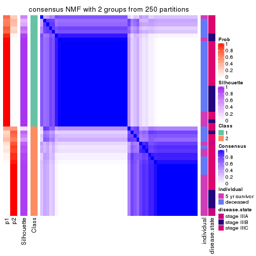
consensus_heatmap(res, k = 3)
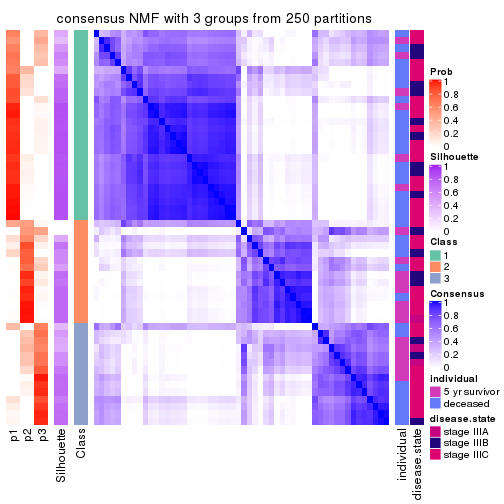
consensus_heatmap(res, k = 4)
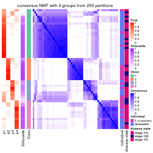
consensus_heatmap(res, k = 5)
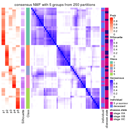
consensus_heatmap(res, k = 6)
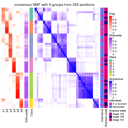
Heatmaps for the membership of samples in all partitions to see how consistent they are:
membership_heatmap(res, k = 2)
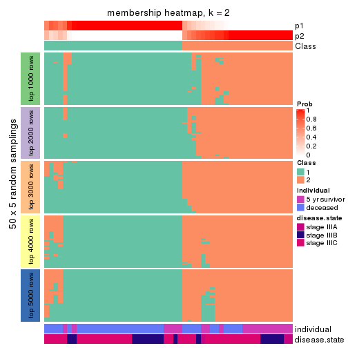
membership_heatmap(res, k = 3)
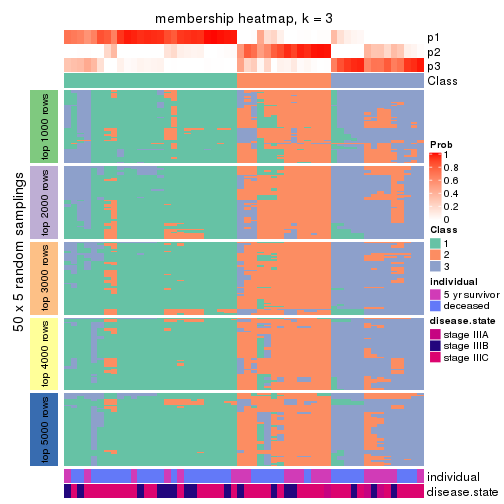
membership_heatmap(res, k = 4)
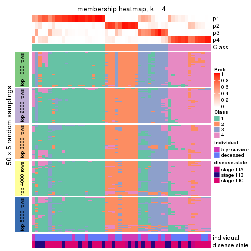
membership_heatmap(res, k = 5)
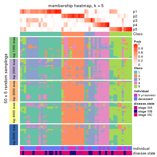
membership_heatmap(res, k = 6)
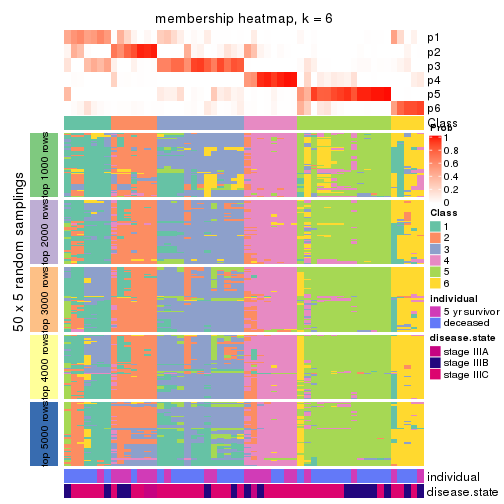
As soon as we have had the classes for columns, we can look for signatures which are significantly different between classes which can be candidate marks for certain classes. Following are the heatmaps for signatures.
Signature heatmaps where rows are scaled:
get_signatures(res, k = 2)
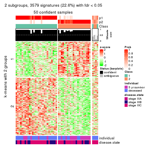
get_signatures(res, k = 3)
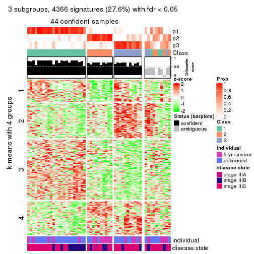
get_signatures(res, k = 4)
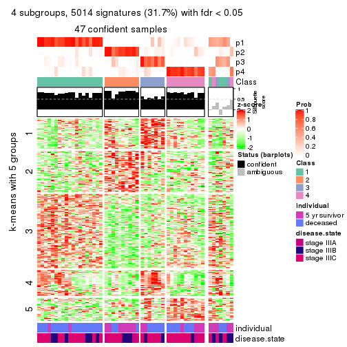
get_signatures(res, k = 5)
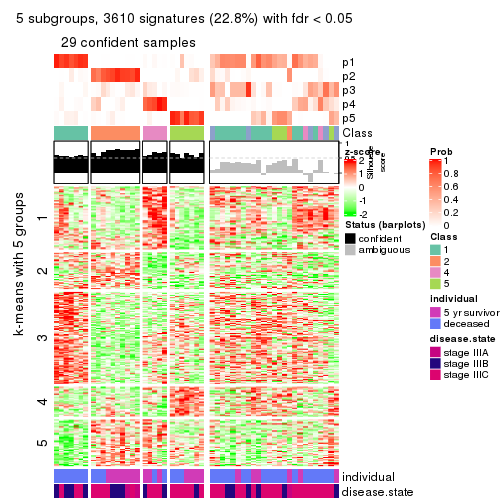
get_signatures(res, k = 6)
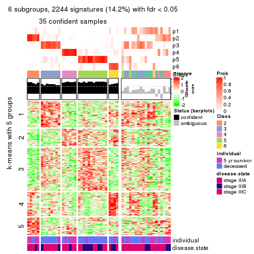
Signature heatmaps where rows are not scaled:
get_signatures(res, k = 2, scale_rows = FALSE)
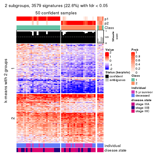
get_signatures(res, k = 3, scale_rows = FALSE)
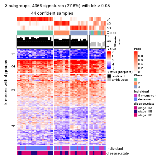
get_signatures(res, k = 4, scale_rows = FALSE)
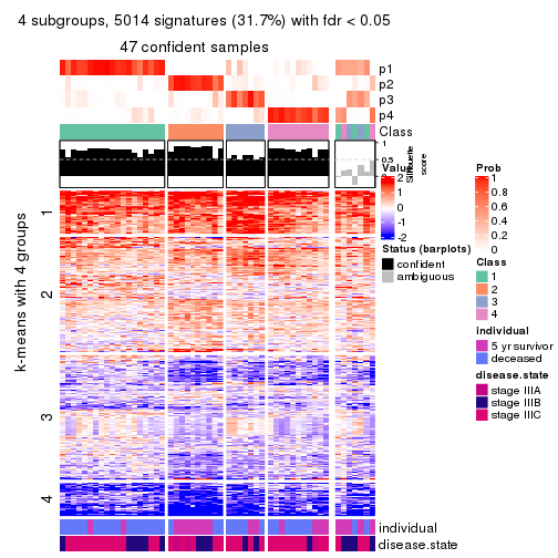
get_signatures(res, k = 5, scale_rows = FALSE)
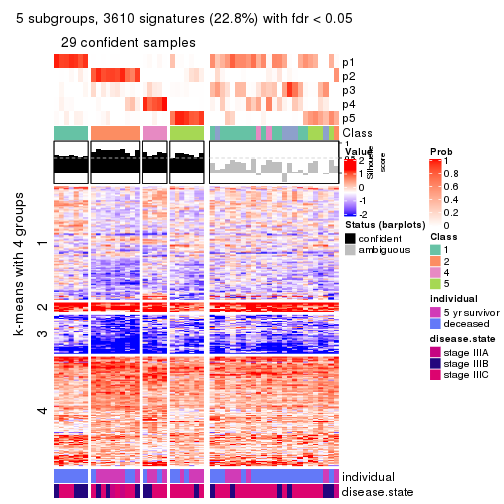
get_signatures(res, k = 6, scale_rows = FALSE)
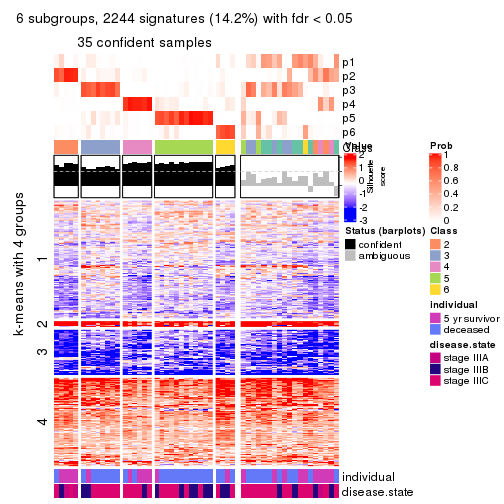
Compare the overlap of signatures from different k:
compare_signatures(res)
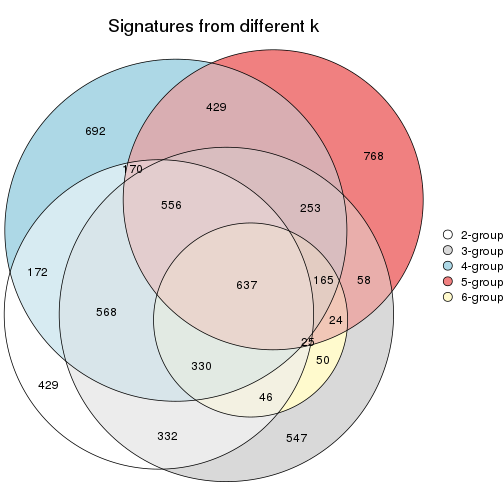
get_signature() returns a data frame invisibly. TO get the list of signatures, the function
call should be assigned to a variable explicitly. In following code, if plot argument is set
to FALSE, no heatmap is plotted while only the differential analysis is performed.
# code only for demonstration
tb = get_signature(res, k = ..., plot = FALSE)
An example of the output of tb is:
#> which_row fdr mean_1 mean_2 scaled_mean_1 scaled_mean_2 km
#> 1 38 0.042760348 8.373488 9.131774 -0.5533452 0.5164555 1
#> 2 40 0.018707592 7.106213 8.469186 -0.6173731 0.5762149 1
#> 3 55 0.019134737 10.221463 11.207825 -0.6159697 0.5749050 1
#> 4 59 0.006059896 5.921854 7.869574 -0.6899429 0.6439467 1
#> 5 60 0.018055526 8.928898 10.211722 -0.6204761 0.5791110 1
#> 6 98 0.009384629 15.714769 14.887706 0.6635654 -0.6193277 2
...
The columns in tb are:
which_row: row indices corresponding to the input matrix.fdr: FDR for the differential test. mean_x: The mean value in group x.scaled_mean_x: The mean value in group x after rows are scaled.km: Row groups if k-means clustering is applied to rows.UMAP plot which shows how samples are separated.
dimension_reduction(res, k = 2, method = "UMAP")
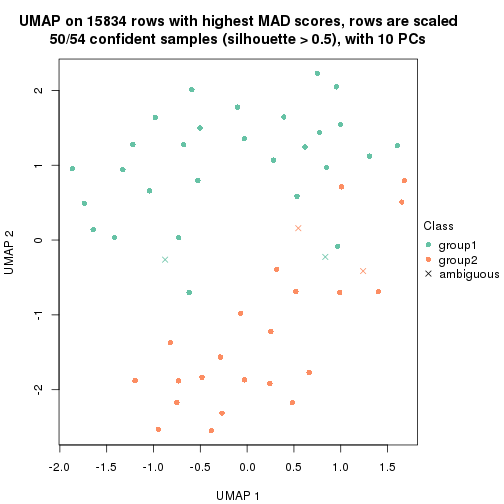
dimension_reduction(res, k = 3, method = "UMAP")
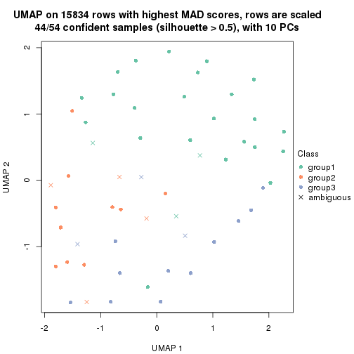
dimension_reduction(res, k = 4, method = "UMAP")
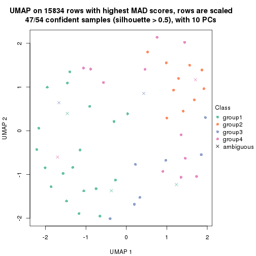
dimension_reduction(res, k = 5, method = "UMAP")
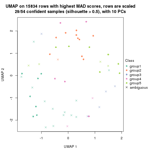
dimension_reduction(res, k = 6, method = "UMAP")
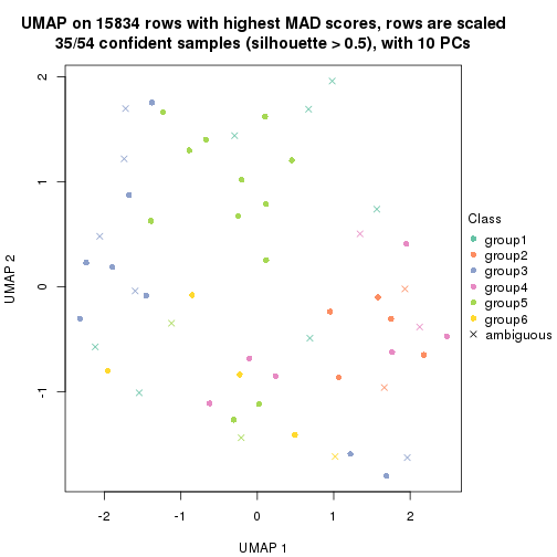
Following heatmap shows how subgroups are split when increasing k:
collect_classes(res)
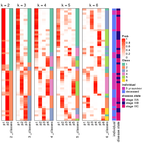
Test correlation between subgroups and known annotations. If the known annotation is numeric, one-way ANOVA test is applied, and if the known annotation is discrete, chi-squared contingency table test is applied.
test_to_known_factors(res)
#> n individual(p) disease.state(p) k
#> MAD:NMF 50 0.00627 0.1258 2
#> MAD:NMF 44 0.02997 0.4884 3
#> MAD:NMF 47 0.01279 0.3183 4
#> MAD:NMF 29 0.03039 0.3140 5
#> MAD:NMF 35 0.00987 0.0479 6
If matrix rows can be associated to genes, consider to use functional_enrichment(res,
...) to perform function enrichment for the signature genes. See this vignette for more detailed explanations.
The object with results only for a single top-value method and a single partition method can be extracted as:
res = res_list["ATC", "hclust"]
# you can also extract it by
# res = res_list["ATC:hclust"]
A summary of res and all the functions that can be applied to it:
res
#> A 'ConsensusPartition' object with k = 2, 3, 4, 5, 6.
#> On a matrix with 15834 rows and 54 columns.
#> Top rows (1000, 2000, 3000, 4000, 5000) are extracted by 'ATC' method.
#> Subgroups are detected by 'hclust' method.
#> Performed in total 1250 partitions by row resampling.
#> Best k for subgroups seems to be 2.
#>
#> Following methods can be applied to this 'ConsensusPartition' object:
#> [1] "cola_report" "collect_classes" "collect_plots"
#> [4] "collect_stats" "colnames" "compare_signatures"
#> [7] "consensus_heatmap" "dimension_reduction" "functional_enrichment"
#> [10] "get_anno_col" "get_anno" "get_classes"
#> [13] "get_consensus" "get_matrix" "get_membership"
#> [16] "get_param" "get_signatures" "get_stats"
#> [19] "is_best_k" "is_stable_k" "membership_heatmap"
#> [22] "ncol" "nrow" "plot_ecdf"
#> [25] "rownames" "select_partition_number" "show"
#> [28] "suggest_best_k" "test_to_known_factors"
collect_plots() function collects all the plots made from res for all k (number of partitions)
into one single page to provide an easy and fast comparison between different k.
collect_plots(res)
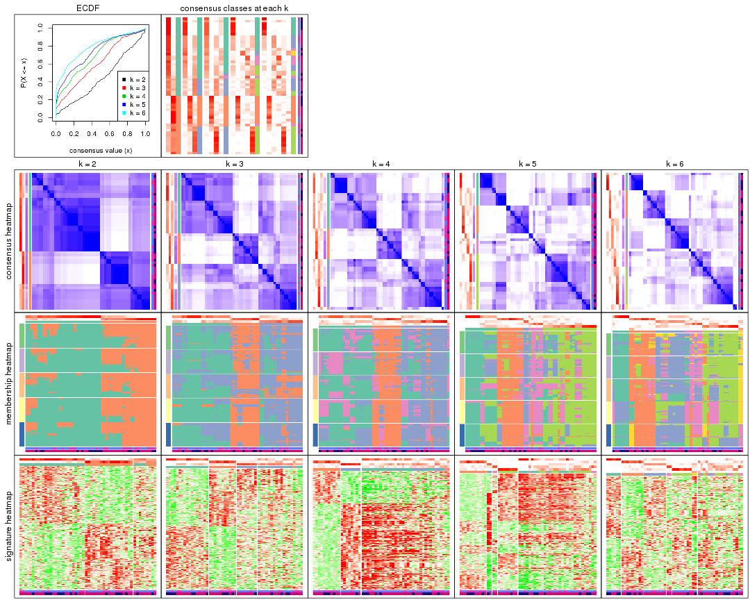
The plots are:
k and the heatmap of
predicted classes for each k.k.k.k.All the plots in panels can be made by individual functions and they are plotted later in this section.
select_partition_number() produces several plots showing different
statistics for choosing “optimized” k. There are following statistics:
k;k, the area increased is defined as \(A_k - A_{k-1}\).The detailed explanations of these statistics can be found in the cola vignette.
Generally speaking, lower PAC score, higher mean silhouette score or higher
concordance corresponds to better partition. Rand index and Jaccard index
measure how similar the current partition is compared to partition with k-1.
If they are too similar, we won't accept k is better than k-1.
select_partition_number(res)
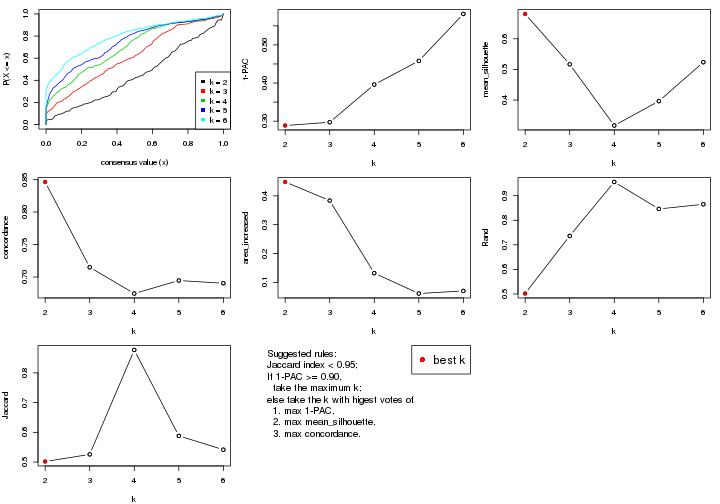
The numeric values for all these statistics can be obtained by get_stats().
get_stats(res)
#> k 1-PAC mean_silhouette concordance area_increased Rand Jaccard
#> 2 2 0.289 0.681 0.846 0.4480 0.502 0.502
#> 3 3 0.297 0.517 0.715 0.3835 0.737 0.526
#> 4 4 0.396 0.317 0.675 0.1318 0.956 0.877
#> 5 5 0.458 0.396 0.695 0.0614 0.846 0.588
#> 6 6 0.581 0.523 0.690 0.0704 0.865 0.542
suggest_best_k() suggests the best \(k\) based on these statistics. The rules are as follows:
suggest_best_k(res)
#> [1] 2
Following shows the table of the partitions (You need to click the show/hide
code output link to see it). The membership matrix (columns with name p*)
is inferred by
clue::cl_consensus()
function with the SE method. Basically the value in the membership matrix
represents the probability to belong to a certain group. The finall class
label for an item is determined with the group with highest probability it
belongs to.
In get_classes() function, the entropy is calculated from the membership
matrix and the silhouette score is calculated from the consensus matrix.
cbind(get_classes(res, k = 2), get_membership(res, k = 2))
#> class entropy silhouette p1 p2
#> GSM311939 2 0.8443 0.645 0.272 0.728
#> GSM311963 2 0.9170 0.514 0.332 0.668
#> GSM311973 1 0.7376 0.712 0.792 0.208
#> GSM311940 2 0.0000 0.740 0.000 1.000
#> GSM311953 2 0.0000 0.740 0.000 1.000
#> GSM311974 2 0.0672 0.741 0.008 0.992
#> GSM311975 1 0.9933 0.128 0.548 0.452
#> GSM311977 2 0.5842 0.721 0.140 0.860
#> GSM311982 1 0.0000 0.819 1.000 0.000
#> GSM311990 2 0.4815 0.740 0.104 0.896
#> GSM311943 1 0.2778 0.822 0.952 0.048
#> GSM311944 1 0.2778 0.822 0.952 0.048
#> GSM311946 2 0.3431 0.745 0.064 0.936
#> GSM311956 2 0.6712 0.703 0.176 0.824
#> GSM311967 2 0.0000 0.740 0.000 1.000
#> GSM311968 2 0.9732 0.471 0.404 0.596
#> GSM311972 1 0.2603 0.823 0.956 0.044
#> GSM311980 1 0.7376 0.712 0.792 0.208
#> GSM311981 1 0.3584 0.816 0.932 0.068
#> GSM311988 2 0.0000 0.740 0.000 1.000
#> GSM311957 1 0.5737 0.774 0.864 0.136
#> GSM311960 1 0.8144 0.639 0.748 0.252
#> GSM311971 1 0.0000 0.819 1.000 0.000
#> GSM311976 1 0.2043 0.823 0.968 0.032
#> GSM311978 1 0.0000 0.819 1.000 0.000
#> GSM311979 1 0.0000 0.819 1.000 0.000
#> GSM311983 1 0.0000 0.819 1.000 0.000
#> GSM311986 2 0.9922 0.359 0.448 0.552
#> GSM311991 1 0.0672 0.821 0.992 0.008
#> GSM311938 2 0.0000 0.740 0.000 1.000
#> GSM311941 2 0.9460 0.543 0.364 0.636
#> GSM311942 2 0.9460 0.543 0.364 0.636
#> GSM311945 1 0.8386 0.611 0.732 0.268
#> GSM311947 2 0.0000 0.740 0.000 1.000
#> GSM311948 2 0.9393 0.555 0.356 0.644
#> GSM311949 1 0.2236 0.823 0.964 0.036
#> GSM311950 2 0.0000 0.740 0.000 1.000
#> GSM311951 2 0.9460 0.543 0.364 0.636
#> GSM311952 1 0.2778 0.822 0.952 0.048
#> GSM311954 2 0.9686 0.476 0.396 0.604
#> GSM311955 1 0.4161 0.804 0.916 0.084
#> GSM311958 1 0.2778 0.822 0.952 0.048
#> GSM311959 1 0.8813 0.481 0.700 0.300
#> GSM311961 1 0.9323 0.431 0.652 0.348
#> GSM311962 1 0.0000 0.819 1.000 0.000
#> GSM311964 1 0.5946 0.780 0.856 0.144
#> GSM311965 2 0.9686 0.476 0.396 0.604
#> GSM311966 1 0.0000 0.819 1.000 0.000
#> GSM311969 1 0.8861 0.473 0.696 0.304
#> GSM311970 1 0.8207 0.645 0.744 0.256
#> GSM311984 1 0.9896 0.175 0.560 0.440
#> GSM311985 1 0.4562 0.811 0.904 0.096
#> GSM311987 2 0.4815 0.740 0.104 0.896
#> GSM311989 1 0.5629 0.777 0.868 0.132
cbind(get_classes(res, k = 3), get_membership(res, k = 3))
#> class entropy silhouette p1 p2 p3
#> GSM311939 3 0.640 0.2734 0.008 0.372 0.620
#> GSM311963 2 0.878 0.2340 0.120 0.512 0.368
#> GSM311973 1 0.779 0.4102 0.524 0.052 0.424
#> GSM311940 2 0.116 0.7825 0.000 0.972 0.028
#> GSM311953 2 0.103 0.7852 0.000 0.976 0.024
#> GSM311974 2 0.334 0.7854 0.000 0.880 0.120
#> GSM311975 3 0.802 0.4038 0.184 0.160 0.656
#> GSM311977 2 0.502 0.6869 0.012 0.796 0.192
#> GSM311982 1 0.116 0.6221 0.972 0.000 0.028
#> GSM311990 3 0.625 -0.0803 0.000 0.444 0.556
#> GSM311943 1 0.611 0.5532 0.604 0.000 0.396
#> GSM311944 1 0.610 0.5560 0.608 0.000 0.392
#> GSM311946 2 0.420 0.7594 0.012 0.852 0.136
#> GSM311956 2 0.584 0.6107 0.016 0.732 0.252
#> GSM311967 2 0.455 0.6969 0.000 0.800 0.200
#> GSM311968 3 0.538 0.6487 0.068 0.112 0.820
#> GSM311972 1 0.614 0.5512 0.596 0.000 0.404
#> GSM311980 1 0.779 0.4102 0.524 0.052 0.424
#> GSM311981 1 0.554 0.5993 0.752 0.012 0.236
#> GSM311988 2 0.435 0.7439 0.000 0.816 0.184
#> GSM311957 1 0.652 0.4391 0.504 0.004 0.492
#> GSM311960 3 0.703 -0.1810 0.368 0.028 0.604
#> GSM311971 1 0.470 0.6427 0.788 0.000 0.212
#> GSM311976 1 0.572 0.6359 0.704 0.004 0.292
#> GSM311978 1 0.116 0.6221 0.972 0.000 0.028
#> GSM311979 1 0.116 0.6221 0.972 0.000 0.028
#> GSM311983 1 0.116 0.6221 0.972 0.000 0.028
#> GSM311986 3 0.610 0.6045 0.120 0.096 0.784
#> GSM311991 1 0.439 0.6365 0.840 0.012 0.148
#> GSM311938 2 0.116 0.7865 0.000 0.972 0.028
#> GSM311941 3 0.414 0.6515 0.020 0.116 0.864
#> GSM311942 3 0.414 0.6515 0.020 0.116 0.864
#> GSM311945 3 0.695 -0.1154 0.352 0.028 0.620
#> GSM311947 2 0.455 0.6969 0.000 0.800 0.200
#> GSM311948 3 0.462 0.6344 0.020 0.144 0.836
#> GSM311949 1 0.569 0.6354 0.708 0.004 0.288
#> GSM311950 2 0.435 0.7439 0.000 0.816 0.184
#> GSM311951 3 0.414 0.6515 0.020 0.116 0.864
#> GSM311952 1 0.611 0.5532 0.604 0.000 0.396
#> GSM311954 3 0.406 0.6584 0.032 0.092 0.876
#> GSM311955 1 0.663 0.4819 0.552 0.008 0.440
#> GSM311958 1 0.610 0.5560 0.608 0.000 0.392
#> GSM311959 3 0.673 0.1739 0.332 0.024 0.644
#> GSM311961 3 0.734 0.2724 0.240 0.080 0.680
#> GSM311962 1 0.164 0.6278 0.956 0.000 0.044
#> GSM311964 1 0.752 0.5119 0.568 0.044 0.388
#> GSM311965 3 0.406 0.6584 0.032 0.092 0.876
#> GSM311966 1 0.129 0.6240 0.968 0.000 0.032
#> GSM311969 3 0.670 0.1843 0.328 0.024 0.648
#> GSM311970 1 0.873 0.3068 0.476 0.108 0.416
#> GSM311984 3 0.791 0.3939 0.188 0.148 0.664
#> GSM311985 1 0.631 0.4387 0.508 0.000 0.492
#> GSM311987 3 0.618 -0.0119 0.000 0.416 0.584
#> GSM311989 1 0.652 0.4561 0.516 0.004 0.480
cbind(get_classes(res, k = 4), get_membership(res, k = 4))
#> class entropy silhouette p1 p2 p3 p4
#> GSM311939 3 0.4868 0.3303 0.000 0.304 0.684 0.012
#> GSM311963 2 0.9090 0.0230 0.144 0.444 0.128 0.284
#> GSM311973 1 0.7971 -0.7911 0.420 0.028 0.140 0.412
#> GSM311940 2 0.0469 0.7440 0.000 0.988 0.000 0.012
#> GSM311953 2 0.1733 0.7566 0.000 0.948 0.024 0.028
#> GSM311974 2 0.2976 0.7498 0.000 0.872 0.120 0.008
#> GSM311975 3 0.8241 0.2467 0.140 0.080 0.552 0.228
#> GSM311977 2 0.5886 0.6355 0.052 0.728 0.036 0.184
#> GSM311982 1 0.3356 0.3501 0.824 0.000 0.000 0.176
#> GSM311990 3 0.6375 0.1816 0.000 0.272 0.624 0.104
#> GSM311943 1 0.5075 0.3648 0.644 0.000 0.344 0.012
#> GSM311944 1 0.5057 0.3691 0.648 0.000 0.340 0.012
#> GSM311946 2 0.4475 0.7298 0.012 0.824 0.068 0.096
#> GSM311956 2 0.6667 0.5619 0.064 0.668 0.048 0.220
#> GSM311967 2 0.5905 0.6087 0.000 0.700 0.156 0.144
#> GSM311968 3 0.1762 0.6200 0.048 0.004 0.944 0.004
#> GSM311972 1 0.5848 0.3509 0.616 0.000 0.336 0.048
#> GSM311980 1 0.7971 -0.7911 0.420 0.028 0.140 0.412
#> GSM311981 1 0.5571 -0.0960 0.580 0.000 0.024 0.396
#> GSM311988 2 0.3668 0.7109 0.000 0.808 0.188 0.004
#> GSM311957 3 0.7500 -0.1497 0.408 0.000 0.412 0.180
#> GSM311960 3 0.7808 -0.1151 0.268 0.008 0.488 0.236
#> GSM311971 1 0.6701 0.2057 0.584 0.000 0.120 0.296
#> GSM311976 1 0.7252 0.1255 0.528 0.000 0.180 0.292
#> GSM311978 1 0.3356 0.3501 0.824 0.000 0.000 0.176
#> GSM311979 1 0.3356 0.3501 0.824 0.000 0.000 0.176
#> GSM311983 1 0.3356 0.3501 0.824 0.000 0.000 0.176
#> GSM311986 3 0.2593 0.5808 0.104 0.004 0.892 0.000
#> GSM311991 1 0.4741 0.0844 0.668 0.000 0.004 0.328
#> GSM311938 2 0.1488 0.7536 0.000 0.956 0.012 0.032
#> GSM311941 3 0.0336 0.6255 0.000 0.008 0.992 0.000
#> GSM311942 3 0.0336 0.6255 0.000 0.008 0.992 0.000
#> GSM311945 3 0.7293 0.0594 0.248 0.004 0.556 0.192
#> GSM311947 2 0.5905 0.6087 0.000 0.700 0.156 0.144
#> GSM311948 3 0.1584 0.6174 0.000 0.036 0.952 0.012
#> GSM311949 1 0.7001 0.0936 0.576 0.000 0.180 0.244
#> GSM311950 2 0.3751 0.7063 0.000 0.800 0.196 0.004
#> GSM311951 3 0.0804 0.6247 0.000 0.008 0.980 0.012
#> GSM311952 1 0.5186 0.3634 0.640 0.000 0.344 0.016
#> GSM311954 3 0.1697 0.6251 0.028 0.004 0.952 0.016
#> GSM311955 1 0.6020 0.2757 0.568 0.000 0.384 0.048
#> GSM311958 1 0.5057 0.3691 0.648 0.000 0.340 0.012
#> GSM311959 3 0.5985 0.2517 0.352 0.000 0.596 0.052
#> GSM311961 3 0.7419 0.2383 0.180 0.008 0.548 0.264
#> GSM311962 1 0.3764 0.3541 0.816 0.000 0.012 0.172
#> GSM311964 1 0.8145 -0.5197 0.452 0.024 0.188 0.336
#> GSM311965 3 0.1697 0.6251 0.028 0.004 0.952 0.016
#> GSM311966 1 0.3539 0.3516 0.820 0.000 0.004 0.176
#> GSM311969 3 0.5970 0.2604 0.348 0.000 0.600 0.052
#> GSM311970 4 0.7653 0.0000 0.364 0.028 0.112 0.496
#> GSM311984 3 0.8169 0.2431 0.148 0.068 0.552 0.232
#> GSM311985 1 0.6435 0.2323 0.532 0.000 0.396 0.072
#> GSM311987 3 0.6042 0.2560 0.000 0.224 0.672 0.104
#> GSM311989 1 0.7499 0.0354 0.420 0.000 0.400 0.180
cbind(get_classes(res, k = 5), get_membership(res, k = 5))
#> class entropy silhouette p1 p2 p3 p4 p5
#> GSM311939 5 0.4193 0.3025 0.000 0.304 0.000 0.012 0.684
#> GSM311963 4 0.5878 -0.2484 0.000 0.428 0.060 0.496 0.016
#> GSM311973 4 0.4175 0.5425 0.096 0.024 0.020 0.824 0.036
#> GSM311940 2 0.0324 0.7477 0.000 0.992 0.004 0.004 0.000
#> GSM311953 2 0.1661 0.7642 0.000 0.940 0.000 0.036 0.024
#> GSM311974 2 0.3096 0.7521 0.000 0.860 0.008 0.024 0.108
#> GSM311975 5 0.6454 0.2636 0.000 0.072 0.044 0.376 0.508
#> GSM311977 2 0.4974 0.6367 0.000 0.720 0.064 0.200 0.016
#> GSM311982 1 0.0404 0.4761 0.988 0.000 0.012 0.000 0.000
#> GSM311990 5 0.6025 0.1493 0.000 0.264 0.092 0.028 0.616
#> GSM311943 1 0.7626 0.2668 0.412 0.000 0.176 0.072 0.340
#> GSM311944 1 0.7621 0.2721 0.416 0.000 0.176 0.072 0.336
#> GSM311946 2 0.3929 0.7330 0.000 0.816 0.016 0.120 0.048
#> GSM311956 2 0.5574 0.5707 0.000 0.660 0.080 0.240 0.020
#> GSM311967 2 0.6347 0.5081 0.000 0.652 0.108 0.092 0.148
#> GSM311968 5 0.1652 0.5800 0.040 0.004 0.008 0.004 0.944
#> GSM311972 1 0.7907 0.2123 0.364 0.000 0.228 0.080 0.328
#> GSM311980 4 0.4175 0.5425 0.096 0.024 0.020 0.824 0.036
#> GSM311981 3 0.4109 0.8664 0.012 0.000 0.764 0.204 0.020
#> GSM311988 2 0.3561 0.7024 0.000 0.796 0.008 0.008 0.188
#> GSM311957 5 0.7458 0.0261 0.216 0.000 0.044 0.332 0.408
#> GSM311960 5 0.6559 0.0105 0.100 0.008 0.016 0.404 0.472
#> GSM311971 1 0.5804 0.0380 0.576 0.000 0.000 0.304 0.120
#> GSM311976 1 0.7108 -0.1685 0.428 0.000 0.032 0.368 0.172
#> GSM311978 1 0.0404 0.4761 0.988 0.000 0.012 0.000 0.000
#> GSM311979 1 0.0404 0.4761 0.988 0.000 0.012 0.000 0.000
#> GSM311983 1 0.0404 0.4761 0.988 0.000 0.012 0.000 0.000
#> GSM311986 5 0.3005 0.5516 0.076 0.004 0.028 0.012 0.880
#> GSM311991 3 0.4237 0.8693 0.076 0.000 0.772 0.152 0.000
#> GSM311938 2 0.1281 0.7609 0.000 0.956 0.000 0.032 0.012
#> GSM311941 5 0.0579 0.5863 0.000 0.008 0.000 0.008 0.984
#> GSM311942 5 0.0579 0.5863 0.000 0.008 0.000 0.008 0.984
#> GSM311945 5 0.6110 0.1778 0.100 0.004 0.008 0.332 0.556
#> GSM311947 2 0.6347 0.5081 0.000 0.652 0.108 0.092 0.148
#> GSM311948 5 0.1364 0.5805 0.000 0.036 0.000 0.012 0.952
#> GSM311949 4 0.7375 0.0317 0.372 0.000 0.052 0.408 0.168
#> GSM311950 2 0.3631 0.6967 0.000 0.788 0.008 0.008 0.196
#> GSM311951 5 0.0693 0.5870 0.000 0.008 0.000 0.012 0.980
#> GSM311952 1 0.7647 0.2633 0.408 0.000 0.180 0.072 0.340
#> GSM311954 5 0.1490 0.5905 0.008 0.004 0.004 0.032 0.952
#> GSM311955 5 0.7833 -0.2208 0.332 0.000 0.216 0.076 0.376
#> GSM311958 1 0.7621 0.2721 0.416 0.000 0.176 0.072 0.336
#> GSM311959 5 0.6805 0.3091 0.116 0.000 0.216 0.080 0.588
#> GSM311961 5 0.6184 0.2469 0.004 0.004 0.104 0.396 0.492
#> GSM311962 1 0.1059 0.4809 0.968 0.000 0.020 0.004 0.008
#> GSM311964 4 0.7053 0.4171 0.104 0.020 0.116 0.620 0.140
#> GSM311965 5 0.1490 0.5905 0.008 0.004 0.004 0.032 0.952
#> GSM311966 1 0.0162 0.4817 0.996 0.000 0.000 0.000 0.004
#> GSM311969 5 0.6780 0.3143 0.116 0.000 0.212 0.080 0.592
#> GSM311970 4 0.3942 0.4113 0.068 0.020 0.088 0.824 0.000
#> GSM311984 5 0.6323 0.2600 0.000 0.060 0.044 0.388 0.508
#> GSM311985 5 0.8209 -0.1572 0.308 0.000 0.196 0.136 0.360
#> GSM311987 5 0.5732 0.2233 0.000 0.216 0.092 0.028 0.664
#> GSM311989 5 0.7502 0.0109 0.228 0.000 0.044 0.332 0.396
cbind(get_classes(res, k = 6), get_membership(res, k = 6))
#> class entropy silhouette p1 p2 p3 p4 p5 p6
#> GSM311939 5 0.3772 0.3890 0.000 0.296 0.004 0.008 0.692 0.000
#> GSM311963 4 0.5980 -0.2712 0.000 0.412 0.084 0.464 0.004 0.036
#> GSM311973 4 0.2648 0.5365 0.000 0.020 0.092 0.876 0.008 0.004
#> GSM311940 2 0.1075 0.7315 0.000 0.952 0.000 0.000 0.000 0.048
#> GSM311953 2 0.1527 0.7438 0.000 0.948 0.020 0.012 0.008 0.012
#> GSM311974 2 0.3369 0.7182 0.000 0.840 0.008 0.020 0.100 0.032
#> GSM311975 3 0.7452 0.2664 0.000 0.072 0.384 0.240 0.284 0.020
#> GSM311977 2 0.4830 0.6408 0.000 0.724 0.056 0.172 0.008 0.040
#> GSM311982 1 0.0000 0.8391 1.000 0.000 0.000 0.000 0.000 0.000
#> GSM311990 5 0.5300 0.3435 0.000 0.252 0.008 0.000 0.612 0.128
#> GSM311943 3 0.5853 0.6471 0.324 0.000 0.544 0.004 0.100 0.028
#> GSM311944 3 0.5865 0.6435 0.328 0.000 0.540 0.004 0.100 0.028
#> GSM311946 2 0.3643 0.7180 0.000 0.836 0.020 0.076 0.028 0.040
#> GSM311956 2 0.5327 0.5740 0.000 0.656 0.060 0.220 0.000 0.064
#> GSM311967 2 0.3899 0.4377 0.000 0.592 0.004 0.000 0.000 0.404
#> GSM311968 5 0.1623 0.6319 0.004 0.000 0.032 0.004 0.940 0.020
#> GSM311972 3 0.5303 0.6422 0.312 0.000 0.584 0.000 0.092 0.012
#> GSM311980 4 0.2648 0.5365 0.000 0.020 0.092 0.876 0.008 0.004
#> GSM311981 6 0.5667 0.8850 0.000 0.000 0.340 0.168 0.000 0.492
#> GSM311988 2 0.4020 0.6543 0.000 0.764 0.008 0.008 0.180 0.040
#> GSM311957 5 0.7211 -0.0703 0.048 0.000 0.148 0.368 0.396 0.040
#> GSM311960 5 0.5505 -0.0216 0.000 0.004 0.084 0.440 0.464 0.008
#> GSM311971 1 0.6825 -0.2326 0.444 0.000 0.080 0.348 0.120 0.008
#> GSM311976 4 0.7843 0.3268 0.260 0.000 0.160 0.408 0.132 0.040
#> GSM311978 1 0.0000 0.8391 1.000 0.000 0.000 0.000 0.000 0.000
#> GSM311979 1 0.0000 0.8391 1.000 0.000 0.000 0.000 0.000 0.000
#> GSM311983 1 0.0000 0.8391 1.000 0.000 0.000 0.000 0.000 0.000
#> GSM311986 5 0.2697 0.5972 0.008 0.000 0.068 0.000 0.876 0.048
#> GSM311991 6 0.6652 0.8846 0.076 0.000 0.352 0.132 0.000 0.440
#> GSM311938 2 0.1621 0.7446 0.000 0.944 0.020 0.008 0.012 0.016
#> GSM311941 5 0.0363 0.6457 0.000 0.000 0.000 0.000 0.988 0.012
#> GSM311942 5 0.0363 0.6457 0.000 0.000 0.000 0.000 0.988 0.012
#> GSM311945 5 0.5147 0.1770 0.008 0.000 0.072 0.364 0.556 0.000
#> GSM311947 2 0.3899 0.4377 0.000 0.592 0.004 0.000 0.000 0.404
#> GSM311948 5 0.1116 0.6442 0.000 0.028 0.004 0.008 0.960 0.000
#> GSM311949 4 0.7755 0.3943 0.204 0.000 0.180 0.444 0.132 0.040
#> GSM311950 2 0.4203 0.6385 0.000 0.740 0.008 0.008 0.204 0.040
#> GSM311951 5 0.0405 0.6444 0.000 0.000 0.004 0.008 0.988 0.000
#> GSM311952 3 0.5785 0.6483 0.324 0.000 0.548 0.004 0.100 0.024
#> GSM311954 5 0.2805 0.5118 0.000 0.000 0.160 0.012 0.828 0.000
#> GSM311955 3 0.5324 0.6666 0.272 0.000 0.592 0.004 0.132 0.000
#> GSM311958 3 0.5865 0.6435 0.328 0.000 0.540 0.004 0.100 0.028
#> GSM311959 3 0.4794 0.5304 0.056 0.000 0.596 0.004 0.344 0.000
#> GSM311961 3 0.6512 0.3201 0.000 0.016 0.472 0.252 0.248 0.012
#> GSM311962 1 0.2113 0.7719 0.908 0.000 0.060 0.000 0.004 0.028
#> GSM311964 4 0.5292 0.4627 0.004 0.016 0.276 0.632 0.064 0.008
#> GSM311965 5 0.2768 0.5177 0.000 0.000 0.156 0.012 0.832 0.000
#> GSM311966 1 0.1049 0.8216 0.960 0.000 0.032 0.000 0.000 0.008
#> GSM311969 3 0.4806 0.5251 0.056 0.000 0.592 0.004 0.348 0.000
#> GSM311970 4 0.2454 0.3560 0.000 0.020 0.088 0.884 0.000 0.008
#> GSM311984 3 0.7364 0.2631 0.000 0.060 0.384 0.252 0.284 0.020
#> GSM311985 3 0.6283 0.6270 0.280 0.000 0.536 0.048 0.132 0.004
#> GSM311987 5 0.5025 0.4094 0.000 0.204 0.008 0.000 0.660 0.128
#> GSM311989 5 0.7322 -0.0913 0.060 0.000 0.144 0.368 0.388 0.040
Heatmaps for the consensus matrix. It visualizes the probability of two samples to be in a same group.
consensus_heatmap(res, k = 2)
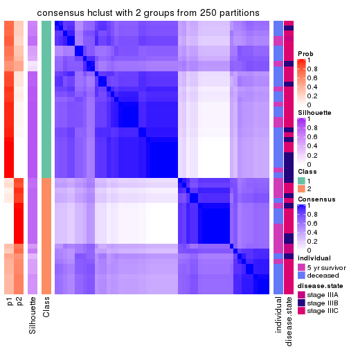
consensus_heatmap(res, k = 3)
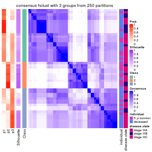
consensus_heatmap(res, k = 4)
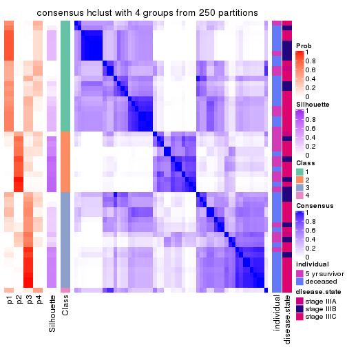
consensus_heatmap(res, k = 5)
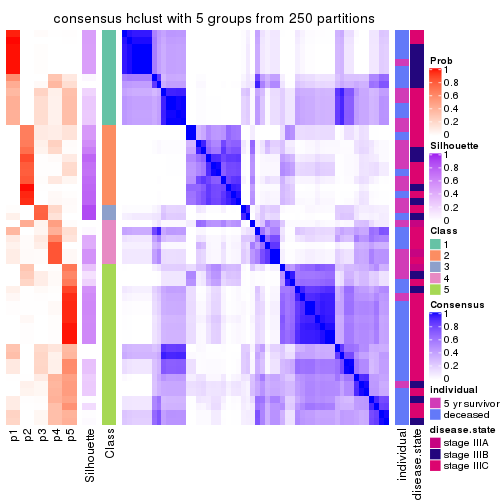
consensus_heatmap(res, k = 6)
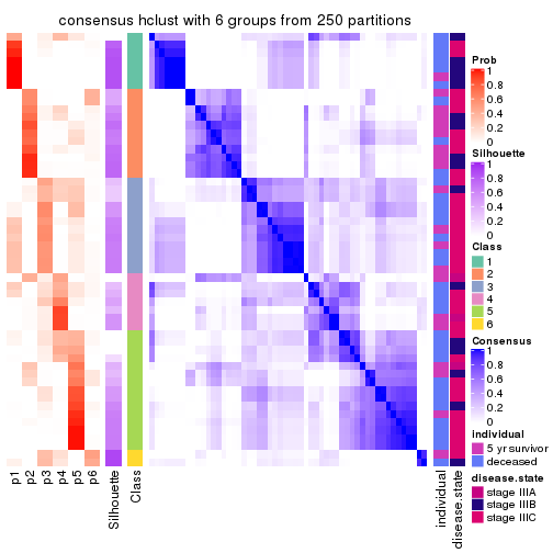
Heatmaps for the membership of samples in all partitions to see how consistent they are:
membership_heatmap(res, k = 2)
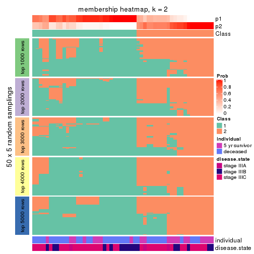
membership_heatmap(res, k = 3)
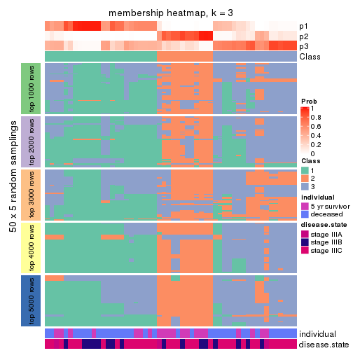
membership_heatmap(res, k = 4)
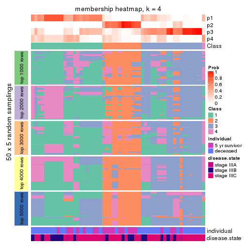
membership_heatmap(res, k = 5)
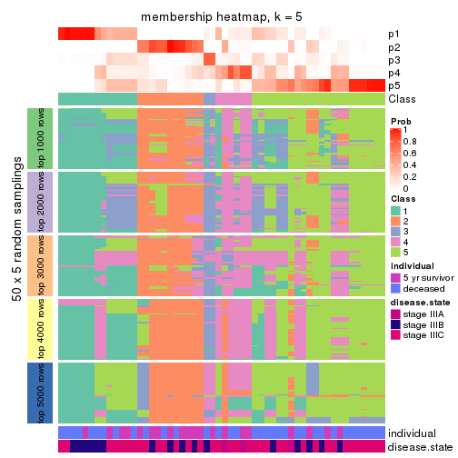
membership_heatmap(res, k = 6)
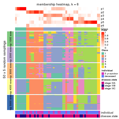
As soon as we have had the classes for columns, we can look for signatures which are significantly different between classes which can be candidate marks for certain classes. Following are the heatmaps for signatures.
Signature heatmaps where rows are scaled:
get_signatures(res, k = 2)
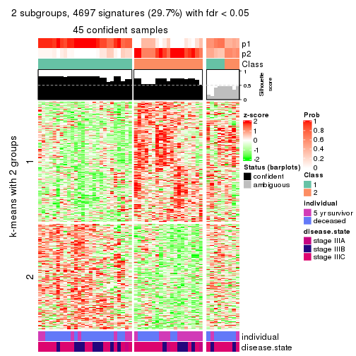
get_signatures(res, k = 3)
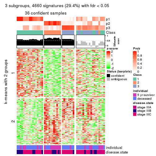
get_signatures(res, k = 4)
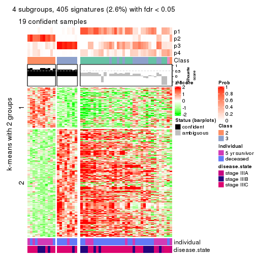
get_signatures(res, k = 5)
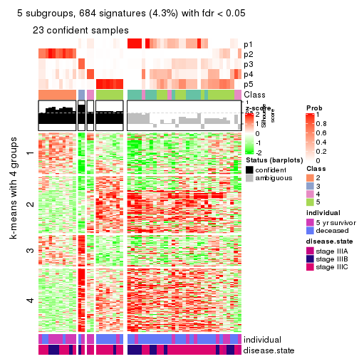
get_signatures(res, k = 6)
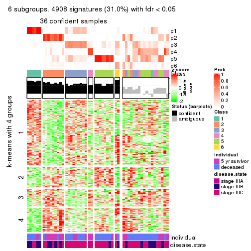
Signature heatmaps where rows are not scaled:
get_signatures(res, k = 2, scale_rows = FALSE)
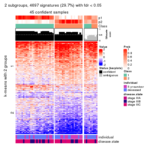
get_signatures(res, k = 3, scale_rows = FALSE)
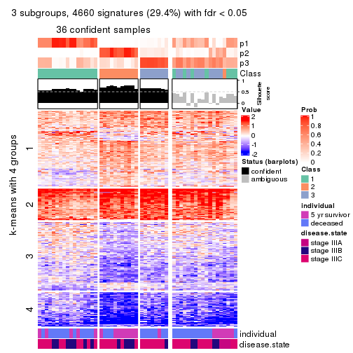
get_signatures(res, k = 4, scale_rows = FALSE)
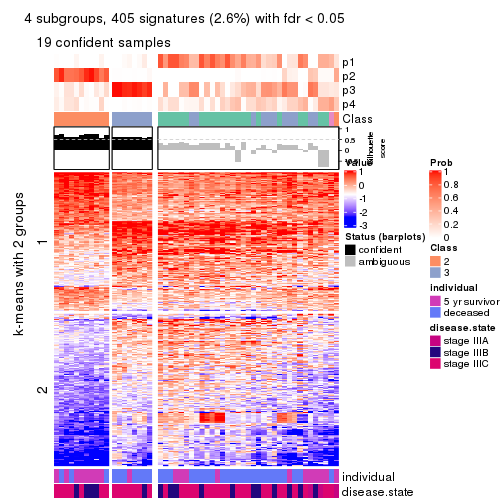
get_signatures(res, k = 5, scale_rows = FALSE)
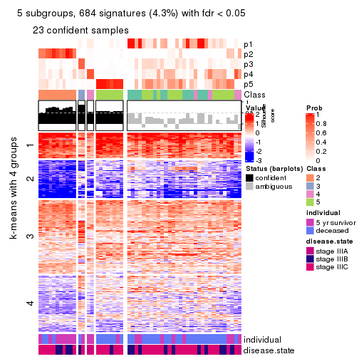
get_signatures(res, k = 6, scale_rows = FALSE)
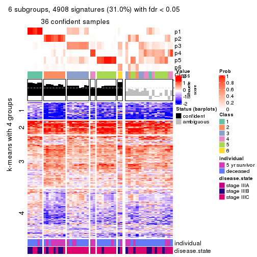
Compare the overlap of signatures from different k:
compare_signatures(res)
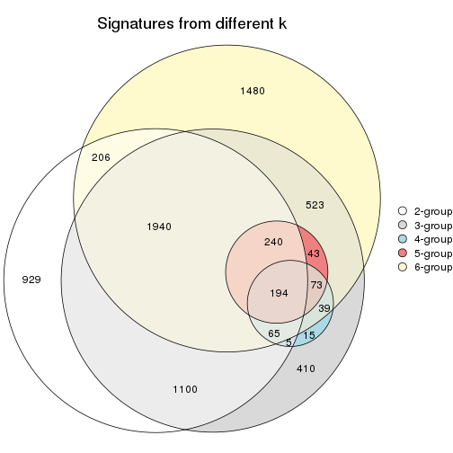
get_signature() returns a data frame invisibly. TO get the list of signatures, the function
call should be assigned to a variable explicitly. In following code, if plot argument is set
to FALSE, no heatmap is plotted while only the differential analysis is performed.
# code only for demonstration
tb = get_signature(res, k = ..., plot = FALSE)
An example of the output of tb is:
#> which_row fdr mean_1 mean_2 scaled_mean_1 scaled_mean_2 km
#> 1 38 0.042760348 8.373488 9.131774 -0.5533452 0.5164555 1
#> 2 40 0.018707592 7.106213 8.469186 -0.6173731 0.5762149 1
#> 3 55 0.019134737 10.221463 11.207825 -0.6159697 0.5749050 1
#> 4 59 0.006059896 5.921854 7.869574 -0.6899429 0.6439467 1
#> 5 60 0.018055526 8.928898 10.211722 -0.6204761 0.5791110 1
#> 6 98 0.009384629 15.714769 14.887706 0.6635654 -0.6193277 2
...
The columns in tb are:
which_row: row indices corresponding to the input matrix.fdr: FDR for the differential test. mean_x: The mean value in group x.scaled_mean_x: The mean value in group x after rows are scaled.km: Row groups if k-means clustering is applied to rows.UMAP plot which shows how samples are separated.
dimension_reduction(res, k = 2, method = "UMAP")
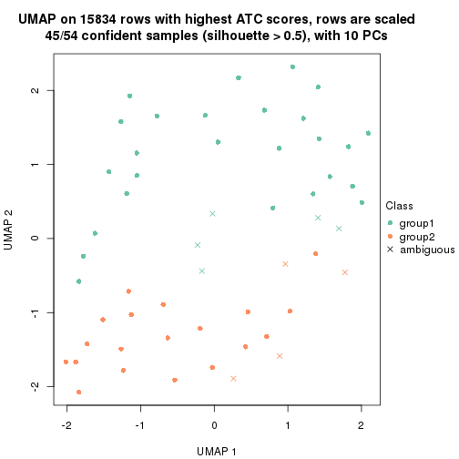
dimension_reduction(res, k = 3, method = "UMAP")
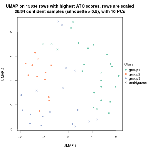
dimension_reduction(res, k = 4, method = "UMAP")
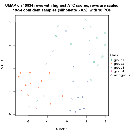
dimension_reduction(res, k = 5, method = "UMAP")
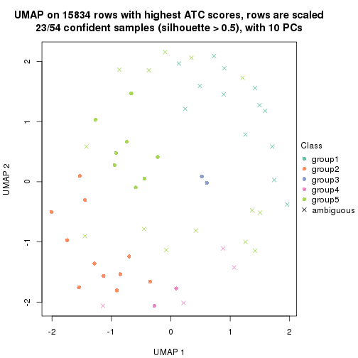
dimension_reduction(res, k = 6, method = "UMAP")
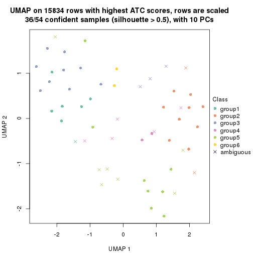
Following heatmap shows how subgroups are split when increasing k:
collect_classes(res)
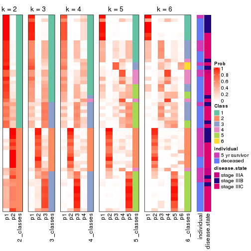
Test correlation between subgroups and known annotations. If the known annotation is numeric, one-way ANOVA test is applied, and if the known annotation is discrete, chi-squared contingency table test is applied.
test_to_known_factors(res)
#> n individual(p) disease.state(p) k
#> ATC:hclust 45 0.0740 0.61186 2
#> ATC:hclust 36 0.0159 0.35371 3
#> ATC:hclust 19 0.0331 0.52303 4
#> ATC:hclust 23 0.0329 0.04121 5
#> ATC:hclust 36 0.0311 0.00154 6
If matrix rows can be associated to genes, consider to use functional_enrichment(res,
...) to perform function enrichment for the signature genes. See this vignette for more detailed explanations.
The object with results only for a single top-value method and a single partition method can be extracted as:
res = res_list["ATC", "kmeans"]
# you can also extract it by
# res = res_list["ATC:kmeans"]
A summary of res and all the functions that can be applied to it:
res
#> A 'ConsensusPartition' object with k = 2, 3, 4, 5, 6.
#> On a matrix with 15834 rows and 54 columns.
#> Top rows (1000, 2000, 3000, 4000, 5000) are extracted by 'ATC' method.
#> Subgroups are detected by 'kmeans' method.
#> Performed in total 1250 partitions by row resampling.
#> Best k for subgroups seems to be 2.
#>
#> Following methods can be applied to this 'ConsensusPartition' object:
#> [1] "cola_report" "collect_classes" "collect_plots"
#> [4] "collect_stats" "colnames" "compare_signatures"
#> [7] "consensus_heatmap" "dimension_reduction" "functional_enrichment"
#> [10] "get_anno_col" "get_anno" "get_classes"
#> [13] "get_consensus" "get_matrix" "get_membership"
#> [16] "get_param" "get_signatures" "get_stats"
#> [19] "is_best_k" "is_stable_k" "membership_heatmap"
#> [22] "ncol" "nrow" "plot_ecdf"
#> [25] "rownames" "select_partition_number" "show"
#> [28] "suggest_best_k" "test_to_known_factors"
collect_plots() function collects all the plots made from res for all k (number of partitions)
into one single page to provide an easy and fast comparison between different k.
collect_plots(res)
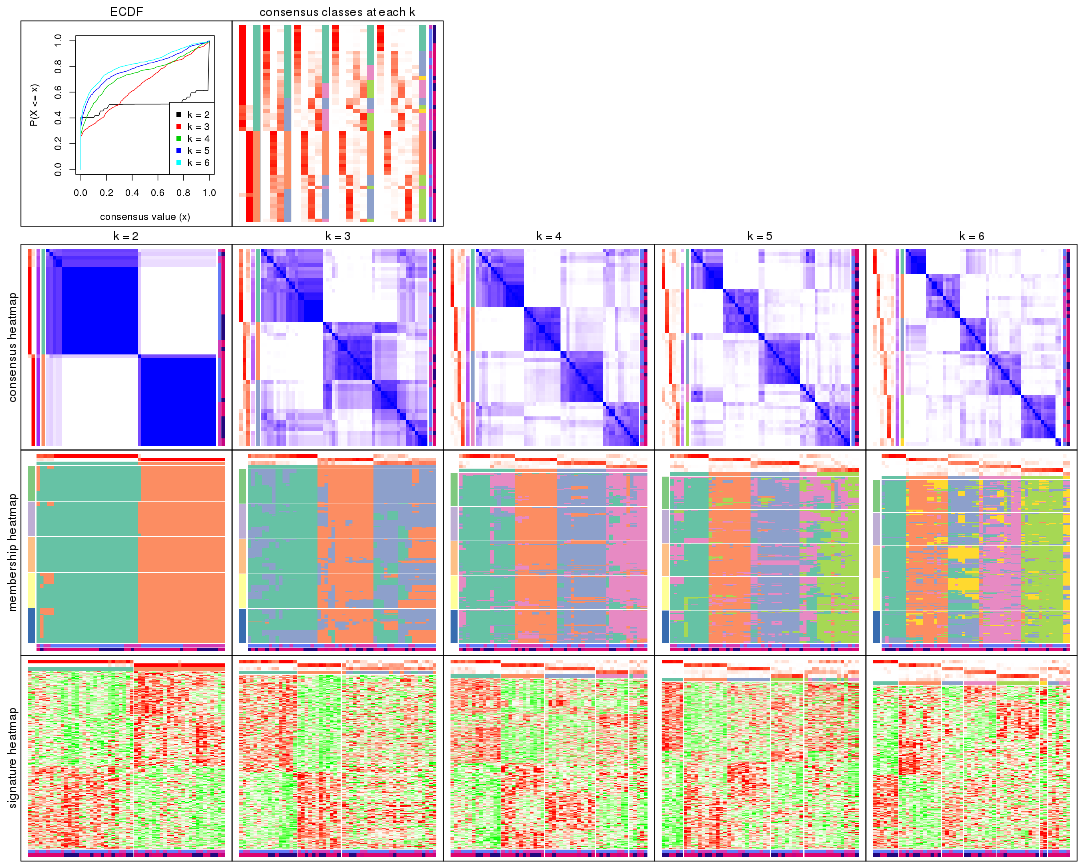
The plots are:
k and the heatmap of
predicted classes for each k.k.k.k.All the plots in panels can be made by individual functions and they are plotted later in this section.
select_partition_number() produces several plots showing different
statistics for choosing “optimized” k. There are following statistics:
k;k, the area increased is defined as \(A_k - A_{k-1}\).The detailed explanations of these statistics can be found in the cola vignette.
Generally speaking, lower PAC score, higher mean silhouette score or higher
concordance corresponds to better partition. Rand index and Jaccard index
measure how similar the current partition is compared to partition with k-1.
If they are too similar, we won't accept k is better than k-1.
select_partition_number(res)
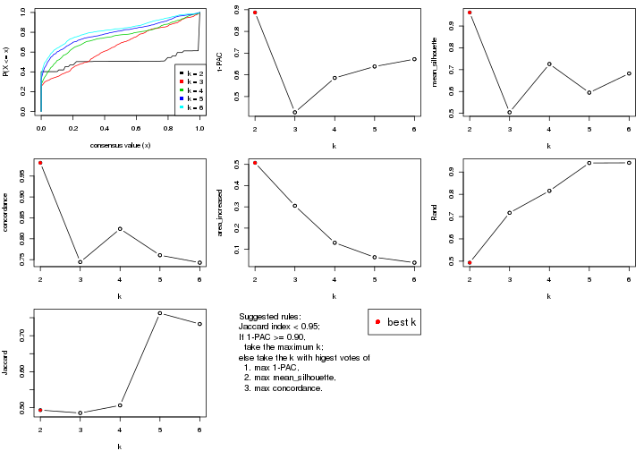
The numeric values for all these statistics can be obtained by get_stats().
get_stats(res)
#> k 1-PAC mean_silhouette concordance area_increased Rand Jaccard
#> 2 2 0.887 0.962 0.982 0.5074 0.493 0.493
#> 3 3 0.427 0.505 0.744 0.3052 0.717 0.485
#> 4 4 0.586 0.726 0.824 0.1309 0.816 0.507
#> 5 5 0.638 0.595 0.761 0.0627 0.941 0.763
#> 6 6 0.672 0.682 0.743 0.0373 0.941 0.732
suggest_best_k() suggests the best \(k\) based on these statistics. The rules are as follows:
suggest_best_k(res)
#> [1] 2
Following shows the table of the partitions (You need to click the show/hide
code output link to see it). The membership matrix (columns with name p*)
is inferred by
clue::cl_consensus()
function with the SE method. Basically the value in the membership matrix
represents the probability to belong to a certain group. The finall class
label for an item is determined with the group with highest probability it
belongs to.
In get_classes() function, the entropy is calculated from the membership
matrix and the silhouette score is calculated from the consensus matrix.
cbind(get_classes(res, k = 2), get_membership(res, k = 2))
#> class entropy silhouette p1 p2
#> GSM311939 2 0.000 0.991 0.000 1.000
#> GSM311963 2 0.000 0.991 0.000 1.000
#> GSM311973 1 0.482 0.886 0.896 0.104
#> GSM311940 2 0.000 0.991 0.000 1.000
#> GSM311953 2 0.000 0.991 0.000 1.000
#> GSM311974 2 0.000 0.991 0.000 1.000
#> GSM311975 2 0.000 0.991 0.000 1.000
#> GSM311977 2 0.000 0.991 0.000 1.000
#> GSM311982 1 0.000 0.972 1.000 0.000
#> GSM311990 2 0.000 0.991 0.000 1.000
#> GSM311943 1 0.000 0.972 1.000 0.000
#> GSM311944 1 0.000 0.972 1.000 0.000
#> GSM311946 2 0.000 0.991 0.000 1.000
#> GSM311956 2 0.000 0.991 0.000 1.000
#> GSM311967 2 0.000 0.991 0.000 1.000
#> GSM311968 2 0.753 0.713 0.216 0.784
#> GSM311972 1 0.000 0.972 1.000 0.000
#> GSM311980 1 0.605 0.843 0.852 0.148
#> GSM311981 1 0.662 0.804 0.828 0.172
#> GSM311988 2 0.000 0.991 0.000 1.000
#> GSM311957 1 0.000 0.972 1.000 0.000
#> GSM311960 2 0.000 0.991 0.000 1.000
#> GSM311971 1 0.000 0.972 1.000 0.000
#> GSM311976 1 0.000 0.972 1.000 0.000
#> GSM311978 1 0.000 0.972 1.000 0.000
#> GSM311979 1 0.000 0.972 1.000 0.000
#> GSM311983 1 0.000 0.972 1.000 0.000
#> GSM311986 1 0.730 0.760 0.796 0.204
#> GSM311991 1 0.000 0.972 1.000 0.000
#> GSM311938 2 0.000 0.991 0.000 1.000
#> GSM311941 2 0.000 0.991 0.000 1.000
#> GSM311942 2 0.000 0.991 0.000 1.000
#> GSM311945 1 0.000 0.972 1.000 0.000
#> GSM311947 2 0.000 0.991 0.000 1.000
#> GSM311948 2 0.000 0.991 0.000 1.000
#> GSM311949 1 0.000 0.972 1.000 0.000
#> GSM311950 2 0.000 0.991 0.000 1.000
#> GSM311951 2 0.000 0.991 0.000 1.000
#> GSM311952 1 0.000 0.972 1.000 0.000
#> GSM311954 2 0.000 0.991 0.000 1.000
#> GSM311955 1 0.000 0.972 1.000 0.000
#> GSM311958 1 0.000 0.972 1.000 0.000
#> GSM311959 1 0.000 0.972 1.000 0.000
#> GSM311961 1 0.000 0.972 1.000 0.000
#> GSM311962 1 0.000 0.972 1.000 0.000
#> GSM311964 1 0.000 0.972 1.000 0.000
#> GSM311965 2 0.000 0.991 0.000 1.000
#> GSM311966 1 0.000 0.972 1.000 0.000
#> GSM311969 1 0.000 0.972 1.000 0.000
#> GSM311970 1 0.605 0.843 0.852 0.148
#> GSM311984 2 0.000 0.991 0.000 1.000
#> GSM311985 1 0.000 0.972 1.000 0.000
#> GSM311987 2 0.000 0.991 0.000 1.000
#> GSM311989 1 0.000 0.972 1.000 0.000
cbind(get_classes(res, k = 3), get_membership(res, k = 3))
#> class entropy silhouette p1 p2 p3
#> GSM311939 2 0.6295 0.09490 0.000 0.528 0.472
#> GSM311963 2 0.6026 0.33977 0.000 0.624 0.376
#> GSM311973 3 0.7739 0.30881 0.188 0.136 0.676
#> GSM311940 2 0.0000 0.78436 0.000 1.000 0.000
#> GSM311953 2 0.0747 0.78509 0.000 0.984 0.016
#> GSM311974 2 0.1031 0.78560 0.000 0.976 0.024
#> GSM311975 2 0.2796 0.77166 0.000 0.908 0.092
#> GSM311977 2 0.1289 0.78059 0.000 0.968 0.032
#> GSM311982 1 0.0000 0.77768 1.000 0.000 0.000
#> GSM311990 3 0.6305 -0.06631 0.000 0.484 0.516
#> GSM311943 1 0.5810 0.49080 0.664 0.000 0.336
#> GSM311944 1 0.3340 0.69728 0.880 0.000 0.120
#> GSM311946 2 0.2537 0.76863 0.000 0.920 0.080
#> GSM311956 2 0.4062 0.63926 0.000 0.836 0.164
#> GSM311967 2 0.2959 0.75020 0.000 0.900 0.100
#> GSM311968 3 0.4504 0.43167 0.000 0.196 0.804
#> GSM311972 1 0.1289 0.77725 0.968 0.000 0.032
#> GSM311980 3 0.7909 0.30395 0.188 0.148 0.664
#> GSM311981 3 0.6669 -0.20505 0.468 0.008 0.524
#> GSM311988 2 0.1411 0.78403 0.000 0.964 0.036
#> GSM311957 1 0.6204 0.44454 0.576 0.000 0.424
#> GSM311960 3 0.5988 0.42769 0.056 0.168 0.776
#> GSM311971 1 0.3267 0.73158 0.884 0.000 0.116
#> GSM311976 1 0.5810 0.56283 0.664 0.000 0.336
#> GSM311978 1 0.0000 0.77768 1.000 0.000 0.000
#> GSM311979 1 0.0000 0.77768 1.000 0.000 0.000
#> GSM311983 1 0.0000 0.77768 1.000 0.000 0.000
#> GSM311986 3 0.4808 0.41832 0.188 0.008 0.804
#> GSM311991 1 0.4452 0.66346 0.808 0.000 0.192
#> GSM311938 2 0.0892 0.78486 0.000 0.980 0.020
#> GSM311941 3 0.5948 0.30885 0.000 0.360 0.640
#> GSM311942 3 0.5835 0.32809 0.000 0.340 0.660
#> GSM311945 3 0.4974 0.23743 0.236 0.000 0.764
#> GSM311947 2 0.3038 0.74702 0.000 0.896 0.104
#> GSM311948 3 0.6267 0.00433 0.000 0.452 0.548
#> GSM311949 1 0.6026 0.53184 0.624 0.000 0.376
#> GSM311950 2 0.2448 0.76499 0.000 0.924 0.076
#> GSM311951 3 0.5785 0.33305 0.000 0.332 0.668
#> GSM311952 1 0.3619 0.72725 0.864 0.000 0.136
#> GSM311954 3 0.5948 0.31493 0.000 0.360 0.640
#> GSM311955 1 0.6252 0.22931 0.556 0.000 0.444
#> GSM311958 1 0.1411 0.77667 0.964 0.000 0.036
#> GSM311959 3 0.6062 0.20039 0.384 0.000 0.616
#> GSM311961 3 0.5968 -0.04229 0.364 0.000 0.636
#> GSM311962 1 0.0000 0.77768 1.000 0.000 0.000
#> GSM311964 1 0.6280 0.42986 0.540 0.000 0.460
#> GSM311965 3 0.5882 0.32830 0.000 0.348 0.652
#> GSM311966 1 0.0000 0.77768 1.000 0.000 0.000
#> GSM311969 3 0.6008 0.22704 0.372 0.000 0.628
#> GSM311970 3 0.7909 0.30395 0.188 0.148 0.664
#> GSM311984 2 0.5835 0.43060 0.000 0.660 0.340
#> GSM311985 1 0.2959 0.75245 0.900 0.000 0.100
#> GSM311987 2 0.6299 0.07724 0.000 0.524 0.476
#> GSM311989 1 0.6062 0.51071 0.616 0.000 0.384
cbind(get_classes(res, k = 4), get_membership(res, k = 4))
#> class entropy silhouette p1 p2 p3 p4
#> GSM311939 3 0.4485 0.8389 0.000 0.152 0.796 0.052
#> GSM311963 4 0.4655 0.4265 0.000 0.312 0.004 0.684
#> GSM311973 4 0.2686 0.7397 0.012 0.040 0.032 0.916
#> GSM311940 2 0.0469 0.9104 0.000 0.988 0.012 0.000
#> GSM311953 2 0.1452 0.9097 0.000 0.956 0.008 0.036
#> GSM311974 2 0.2589 0.9046 0.000 0.912 0.044 0.044
#> GSM311975 2 0.3745 0.8654 0.000 0.852 0.060 0.088
#> GSM311977 2 0.2345 0.8838 0.000 0.900 0.000 0.100
#> GSM311982 1 0.0469 0.7729 0.988 0.000 0.000 0.012
#> GSM311990 3 0.3479 0.8428 0.000 0.148 0.840 0.012
#> GSM311943 1 0.6019 0.6402 0.672 0.000 0.228 0.100
#> GSM311944 1 0.2489 0.7654 0.912 0.000 0.068 0.020
#> GSM311946 2 0.3937 0.8086 0.000 0.800 0.012 0.188
#> GSM311956 2 0.3249 0.8463 0.000 0.852 0.008 0.140
#> GSM311967 2 0.2081 0.8839 0.000 0.916 0.084 0.000
#> GSM311968 3 0.3399 0.8225 0.000 0.040 0.868 0.092
#> GSM311972 1 0.5091 0.7069 0.752 0.000 0.068 0.180
#> GSM311980 4 0.2376 0.7340 0.000 0.068 0.016 0.916
#> GSM311981 4 0.7078 0.4706 0.180 0.032 0.144 0.644
#> GSM311988 2 0.2675 0.9036 0.000 0.908 0.048 0.044
#> GSM311957 4 0.6821 0.4695 0.256 0.000 0.152 0.592
#> GSM311960 4 0.5619 0.5929 0.000 0.064 0.248 0.688
#> GSM311971 1 0.3751 0.5721 0.800 0.000 0.004 0.196
#> GSM311976 4 0.4401 0.5838 0.272 0.000 0.004 0.724
#> GSM311978 1 0.0188 0.7733 0.996 0.000 0.000 0.004
#> GSM311979 1 0.0469 0.7729 0.988 0.000 0.000 0.012
#> GSM311983 1 0.0188 0.7739 0.996 0.000 0.000 0.004
#> GSM311986 3 0.3700 0.7981 0.036 0.012 0.864 0.088
#> GSM311991 1 0.6673 0.0484 0.464 0.004 0.072 0.460
#> GSM311938 2 0.0817 0.9093 0.000 0.976 0.024 0.000
#> GSM311941 3 0.2843 0.8671 0.000 0.088 0.892 0.020
#> GSM311942 3 0.2984 0.8656 0.000 0.084 0.888 0.028
#> GSM311945 4 0.5391 0.6662 0.052 0.008 0.208 0.732
#> GSM311947 2 0.2081 0.8839 0.000 0.916 0.084 0.000
#> GSM311948 3 0.4234 0.8515 0.000 0.132 0.816 0.052
#> GSM311949 4 0.4511 0.5858 0.268 0.000 0.008 0.724
#> GSM311950 2 0.2053 0.8897 0.000 0.924 0.072 0.004
#> GSM311951 3 0.3082 0.8635 0.000 0.084 0.884 0.032
#> GSM311952 1 0.5174 0.7201 0.760 0.000 0.116 0.124
#> GSM311954 3 0.2401 0.8630 0.000 0.092 0.904 0.004
#> GSM311955 1 0.6616 0.5311 0.584 0.000 0.308 0.108
#> GSM311958 1 0.4318 0.7434 0.816 0.000 0.068 0.116
#> GSM311959 3 0.5030 0.5843 0.188 0.000 0.752 0.060
#> GSM311961 4 0.4161 0.7100 0.056 0.004 0.108 0.832
#> GSM311962 1 0.0469 0.7739 0.988 0.000 0.000 0.012
#> GSM311964 4 0.3519 0.7100 0.120 0.004 0.020 0.856
#> GSM311965 3 0.2266 0.8643 0.000 0.084 0.912 0.004
#> GSM311966 1 0.0336 0.7738 0.992 0.000 0.000 0.008
#> GSM311969 3 0.4379 0.6351 0.172 0.000 0.792 0.036
#> GSM311970 4 0.2485 0.7319 0.004 0.064 0.016 0.916
#> GSM311984 3 0.5713 0.5448 0.000 0.340 0.620 0.040
#> GSM311985 1 0.5248 0.7114 0.748 0.000 0.088 0.164
#> GSM311987 3 0.3591 0.8252 0.000 0.168 0.824 0.008
#> GSM311989 1 0.7335 0.0322 0.444 0.000 0.156 0.400
cbind(get_classes(res, k = 5), get_membership(res, k = 5))
#> class entropy silhouette p1 p2 p3 p4 p5
#> GSM311939 3 0.3815 0.7611 0.000 0.060 0.832 0.088 0.020
#> GSM311963 5 0.5564 0.4092 0.000 0.200 0.008 0.128 0.664
#> GSM311973 5 0.1202 0.6682 0.004 0.000 0.032 0.004 0.960
#> GSM311940 2 0.0898 0.8672 0.000 0.972 0.000 0.020 0.008
#> GSM311953 2 0.1918 0.8703 0.000 0.928 0.000 0.036 0.036
#> GSM311974 2 0.4189 0.8442 0.000 0.812 0.044 0.100 0.044
#> GSM311975 2 0.4292 0.7994 0.000 0.788 0.048 0.144 0.020
#> GSM311977 2 0.2992 0.8573 0.000 0.868 0.000 0.064 0.068
#> GSM311982 1 0.0290 0.6750 0.992 0.000 0.000 0.008 0.000
#> GSM311990 3 0.2899 0.7974 0.000 0.036 0.880 0.076 0.008
#> GSM311943 1 0.7308 -0.3079 0.396 0.000 0.164 0.392 0.048
#> GSM311944 1 0.4070 0.3799 0.728 0.000 0.012 0.256 0.004
#> GSM311946 2 0.6238 0.6883 0.000 0.624 0.032 0.140 0.204
#> GSM311956 2 0.3346 0.8464 0.000 0.844 0.000 0.064 0.092
#> GSM311967 2 0.2429 0.8435 0.000 0.900 0.020 0.076 0.004
#> GSM311968 3 0.1701 0.7953 0.000 0.000 0.936 0.016 0.048
#> GSM311972 4 0.4990 0.3680 0.384 0.000 0.000 0.580 0.036
#> GSM311980 5 0.1168 0.6562 0.000 0.008 0.000 0.032 0.960
#> GSM311981 4 0.5159 0.2601 0.020 0.024 0.016 0.696 0.244
#> GSM311988 2 0.4747 0.8251 0.000 0.776 0.072 0.108 0.044
#> GSM311957 5 0.6782 0.5658 0.148 0.000 0.112 0.128 0.612
#> GSM311960 5 0.4655 0.5753 0.000 0.012 0.244 0.032 0.712
#> GSM311971 1 0.3197 0.4716 0.832 0.000 0.004 0.012 0.152
#> GSM311976 5 0.4763 0.6214 0.152 0.000 0.004 0.104 0.740
#> GSM311978 1 0.0162 0.6777 0.996 0.000 0.000 0.004 0.000
#> GSM311979 1 0.0290 0.6750 0.992 0.000 0.000 0.008 0.000
#> GSM311983 1 0.0162 0.6777 0.996 0.000 0.000 0.004 0.000
#> GSM311986 3 0.2450 0.7870 0.000 0.000 0.900 0.052 0.048
#> GSM311991 4 0.5981 0.4214 0.196 0.000 0.000 0.588 0.216
#> GSM311938 2 0.0865 0.8658 0.000 0.972 0.004 0.024 0.000
#> GSM311941 3 0.0566 0.8109 0.000 0.004 0.984 0.012 0.000
#> GSM311942 3 0.0807 0.8067 0.000 0.000 0.976 0.012 0.012
#> GSM311945 5 0.5553 0.6131 0.016 0.000 0.164 0.136 0.684
#> GSM311947 2 0.2429 0.8435 0.000 0.900 0.020 0.076 0.004
#> GSM311948 3 0.3240 0.7843 0.000 0.036 0.868 0.072 0.024
#> GSM311949 5 0.4999 0.6165 0.148 0.000 0.004 0.128 0.720
#> GSM311950 2 0.3523 0.8478 0.000 0.836 0.040 0.116 0.008
#> GSM311951 3 0.1117 0.8059 0.000 0.000 0.964 0.020 0.016
#> GSM311952 1 0.6498 -0.0955 0.516 0.000 0.068 0.364 0.052
#> GSM311954 3 0.2818 0.7859 0.000 0.012 0.856 0.132 0.000
#> GSM311955 4 0.7367 0.1182 0.364 0.000 0.188 0.404 0.044
#> GSM311958 1 0.5525 0.0213 0.576 0.000 0.016 0.364 0.044
#> GSM311959 3 0.6504 0.0684 0.096 0.000 0.464 0.412 0.028
#> GSM311961 5 0.5083 0.3836 0.004 0.000 0.028 0.428 0.540
#> GSM311962 1 0.0703 0.6691 0.976 0.000 0.000 0.024 0.000
#> GSM311964 5 0.4394 0.6104 0.048 0.000 0.000 0.220 0.732
#> GSM311965 3 0.2462 0.7905 0.000 0.008 0.880 0.112 0.000
#> GSM311966 1 0.0162 0.6777 0.996 0.000 0.000 0.004 0.000
#> GSM311969 3 0.5971 0.1499 0.096 0.000 0.496 0.404 0.004
#> GSM311970 5 0.2130 0.6343 0.000 0.012 0.000 0.080 0.908
#> GSM311984 3 0.5006 0.6334 0.000 0.180 0.704 0.116 0.000
#> GSM311985 4 0.5617 0.2780 0.424 0.000 0.012 0.516 0.048
#> GSM311987 3 0.3752 0.7798 0.000 0.044 0.812 0.140 0.004
#> GSM311989 5 0.7985 0.2423 0.264 0.000 0.124 0.184 0.428
cbind(get_classes(res, k = 6), get_membership(res, k = 6))
#> class entropy silhouette p1 p2 p3 p4 p5 p6
#> GSM311939 5 0.3512 0.750 0.000 0.040 0.012 0.000 0.808 0.140
#> GSM311963 4 0.5578 0.216 0.000 0.144 0.000 0.536 0.004 0.316
#> GSM311973 4 0.1672 0.603 0.000 0.000 0.016 0.932 0.004 0.048
#> GSM311940 2 0.0146 0.749 0.000 0.996 0.000 0.000 0.000 0.004
#> GSM311953 2 0.2692 0.761 0.000 0.840 0.000 0.012 0.000 0.148
#> GSM311974 2 0.4967 0.719 0.000 0.668 0.004 0.020 0.064 0.244
#> GSM311975 2 0.5504 0.606 0.000 0.668 0.068 0.012 0.056 0.196
#> GSM311977 2 0.4033 0.737 0.000 0.724 0.000 0.052 0.000 0.224
#> GSM311982 1 0.0000 0.935 1.000 0.000 0.000 0.000 0.000 0.000
#> GSM311990 5 0.2817 0.816 0.000 0.008 0.052 0.000 0.868 0.072
#> GSM311943 3 0.4200 0.677 0.164 0.000 0.744 0.004 0.088 0.000
#> GSM311944 3 0.4234 0.499 0.440 0.000 0.544 0.000 0.016 0.000
#> GSM311946 2 0.6833 0.553 0.000 0.452 0.004 0.148 0.076 0.320
#> GSM311956 2 0.4134 0.730 0.000 0.708 0.000 0.052 0.000 0.240
#> GSM311967 2 0.3190 0.685 0.000 0.844 0.056 0.000 0.012 0.088
#> GSM311968 5 0.2466 0.806 0.000 0.000 0.052 0.028 0.896 0.024
#> GSM311972 3 0.5148 0.427 0.196 0.000 0.624 0.000 0.000 0.180
#> GSM311980 4 0.1765 0.576 0.000 0.000 0.000 0.904 0.000 0.096
#> GSM311981 6 0.5789 0.812 0.000 0.008 0.316 0.128 0.008 0.540
#> GSM311988 2 0.5628 0.682 0.000 0.612 0.008 0.020 0.112 0.248
#> GSM311957 4 0.6256 0.563 0.064 0.000 0.224 0.600 0.088 0.024
#> GSM311960 4 0.4703 0.540 0.000 0.000 0.028 0.704 0.208 0.060
#> GSM311971 1 0.1714 0.821 0.908 0.000 0.000 0.092 0.000 0.000
#> GSM311976 4 0.4528 0.605 0.080 0.000 0.144 0.744 0.000 0.032
#> GSM311978 1 0.0260 0.936 0.992 0.000 0.008 0.000 0.000 0.000
#> GSM311979 1 0.0000 0.935 1.000 0.000 0.000 0.000 0.000 0.000
#> GSM311983 1 0.0260 0.936 0.992 0.000 0.008 0.000 0.000 0.000
#> GSM311986 5 0.4184 0.700 0.000 0.000 0.196 0.032 0.744 0.028
#> GSM311991 6 0.6662 0.798 0.076 0.000 0.340 0.136 0.000 0.448
#> GSM311938 2 0.0692 0.745 0.000 0.976 0.000 0.000 0.004 0.020
#> GSM311941 5 0.0632 0.836 0.000 0.000 0.024 0.000 0.976 0.000
#> GSM311942 5 0.0972 0.834 0.000 0.000 0.028 0.000 0.964 0.008
#> GSM311945 4 0.5254 0.603 0.000 0.000 0.200 0.660 0.112 0.028
#> GSM311947 2 0.3190 0.685 0.000 0.844 0.056 0.000 0.012 0.088
#> GSM311948 5 0.2174 0.809 0.000 0.008 0.008 0.000 0.896 0.088
#> GSM311949 4 0.4465 0.611 0.060 0.000 0.168 0.744 0.004 0.024
#> GSM311950 2 0.4646 0.715 0.000 0.700 0.032 0.000 0.044 0.224
#> GSM311951 5 0.1401 0.833 0.000 0.000 0.028 0.004 0.948 0.020
#> GSM311952 3 0.4892 0.662 0.280 0.000 0.648 0.032 0.040 0.000
#> GSM311954 5 0.3812 0.772 0.000 0.004 0.168 0.000 0.772 0.056
#> GSM311955 3 0.4213 0.675 0.160 0.000 0.744 0.004 0.092 0.000
#> GSM311958 3 0.3850 0.638 0.340 0.000 0.652 0.004 0.000 0.004
#> GSM311959 3 0.4364 0.505 0.040 0.000 0.724 0.004 0.216 0.016
#> GSM311961 4 0.5855 0.386 0.000 0.000 0.220 0.576 0.024 0.180
#> GSM311962 1 0.2346 0.767 0.868 0.000 0.124 0.008 0.000 0.000
#> GSM311964 4 0.4734 0.558 0.016 0.000 0.160 0.720 0.004 0.100
#> GSM311965 5 0.3163 0.797 0.000 0.000 0.140 0.000 0.820 0.040
#> GSM311966 1 0.0260 0.936 0.992 0.000 0.008 0.000 0.000 0.000
#> GSM311969 3 0.4773 0.434 0.036 0.000 0.672 0.000 0.256 0.036
#> GSM311970 4 0.1806 0.570 0.000 0.000 0.004 0.908 0.000 0.088
#> GSM311984 5 0.5343 0.636 0.000 0.084 0.040 0.004 0.664 0.208
#> GSM311985 3 0.4895 0.564 0.256 0.000 0.636 0.000 0.000 0.108
#> GSM311987 5 0.4574 0.742 0.000 0.012 0.148 0.000 0.724 0.116
#> GSM311989 4 0.6951 0.361 0.076 0.000 0.364 0.436 0.100 0.024
Heatmaps for the consensus matrix. It visualizes the probability of two samples to be in a same group.
consensus_heatmap(res, k = 2)
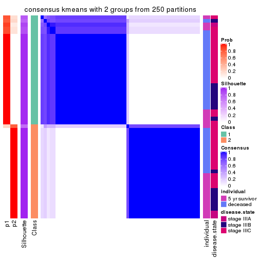
consensus_heatmap(res, k = 3)
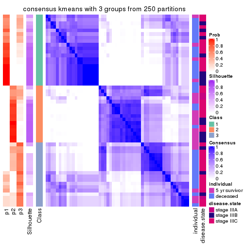
consensus_heatmap(res, k = 4)
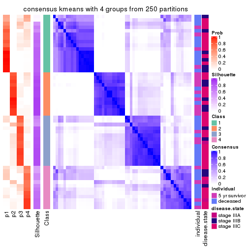
consensus_heatmap(res, k = 5)
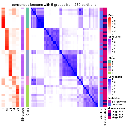
consensus_heatmap(res, k = 6)
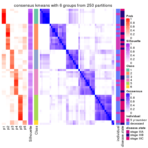
Heatmaps for the membership of samples in all partitions to see how consistent they are:
membership_heatmap(res, k = 2)

membership_heatmap(res, k = 3)
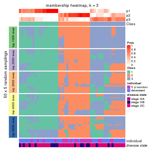
membership_heatmap(res, k = 4)
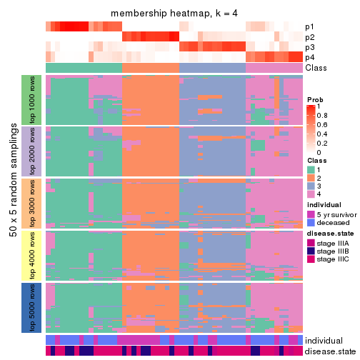
membership_heatmap(res, k = 5)
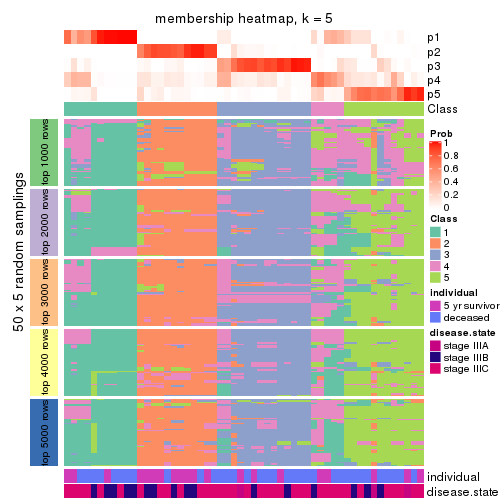
membership_heatmap(res, k = 6)
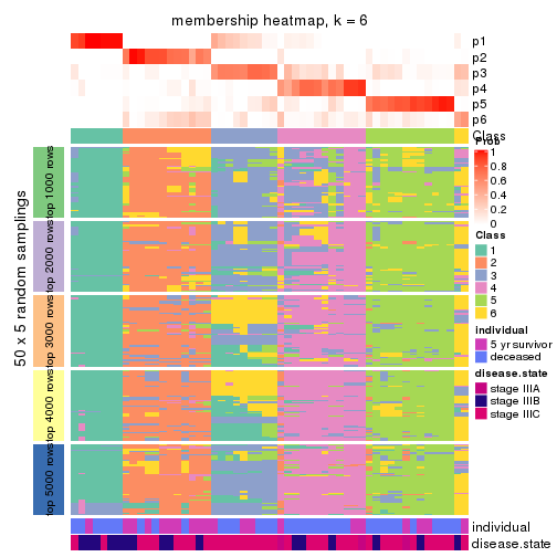
As soon as we have had the classes for columns, we can look for signatures which are significantly different between classes which can be candidate marks for certain classes. Following are the heatmaps for signatures.
Signature heatmaps where rows are scaled:
get_signatures(res, k = 2)
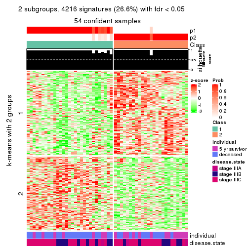
get_signatures(res, k = 3)
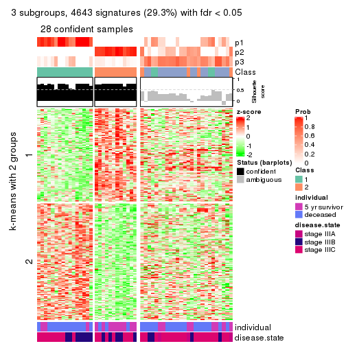
get_signatures(res, k = 4)
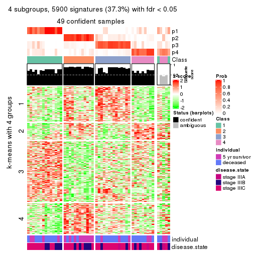
get_signatures(res, k = 5)
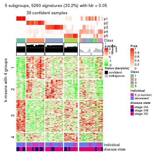
get_signatures(res, k = 6)
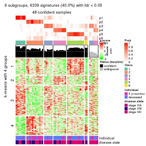
Signature heatmaps where rows are not scaled:
get_signatures(res, k = 2, scale_rows = FALSE)
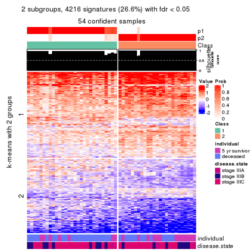
get_signatures(res, k = 3, scale_rows = FALSE)
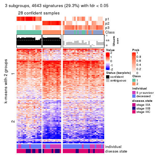
get_signatures(res, k = 4, scale_rows = FALSE)
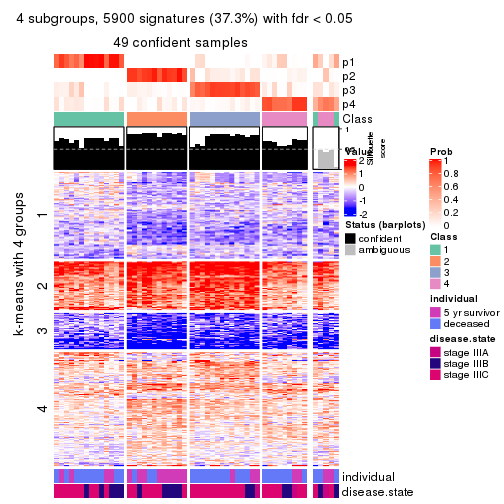
get_signatures(res, k = 5, scale_rows = FALSE)
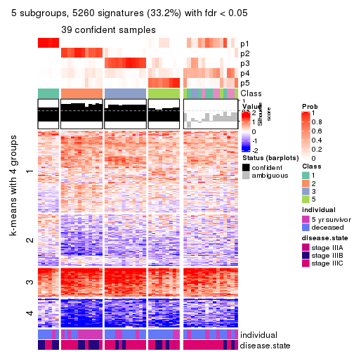
get_signatures(res, k = 6, scale_rows = FALSE)
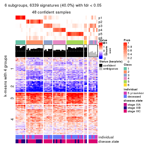
Compare the overlap of signatures from different k:
compare_signatures(res)
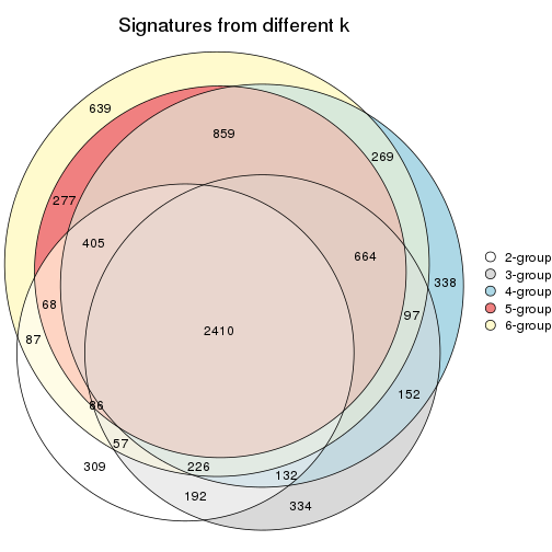
get_signature() returns a data frame invisibly. TO get the list of signatures, the function
call should be assigned to a variable explicitly. In following code, if plot argument is set
to FALSE, no heatmap is plotted while only the differential analysis is performed.
# code only for demonstration
tb = get_signature(res, k = ..., plot = FALSE)
An example of the output of tb is:
#> which_row fdr mean_1 mean_2 scaled_mean_1 scaled_mean_2 km
#> 1 38 0.042760348 8.373488 9.131774 -0.5533452 0.5164555 1
#> 2 40 0.018707592 7.106213 8.469186 -0.6173731 0.5762149 1
#> 3 55 0.019134737 10.221463 11.207825 -0.6159697 0.5749050 1
#> 4 59 0.006059896 5.921854 7.869574 -0.6899429 0.6439467 1
#> 5 60 0.018055526 8.928898 10.211722 -0.6204761 0.5791110 1
#> 6 98 0.009384629 15.714769 14.887706 0.6635654 -0.6193277 2
...
The columns in tb are:
which_row: row indices corresponding to the input matrix.fdr: FDR for the differential test. mean_x: The mean value in group x.scaled_mean_x: The mean value in group x after rows are scaled.km: Row groups if k-means clustering is applied to rows.UMAP plot which shows how samples are separated.
dimension_reduction(res, k = 2, method = "UMAP")

dimension_reduction(res, k = 3, method = "UMAP")
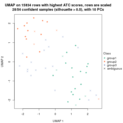
dimension_reduction(res, k = 4, method = "UMAP")
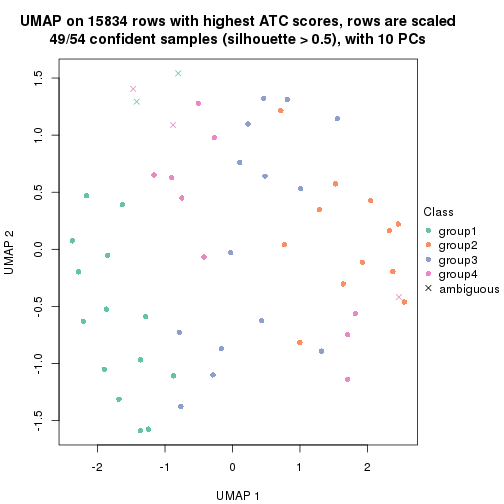
dimension_reduction(res, k = 5, method = "UMAP")
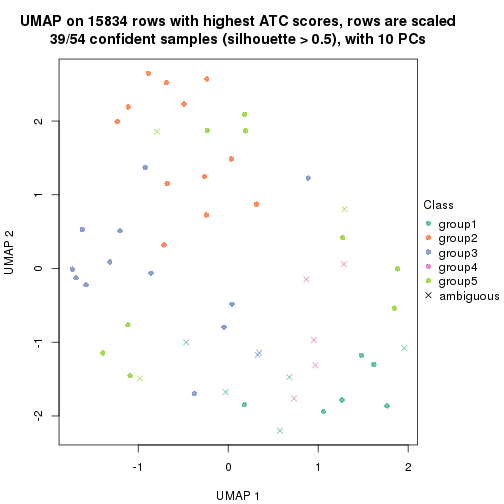
dimension_reduction(res, k = 6, method = "UMAP")

Following heatmap shows how subgroups are split when increasing k:
collect_classes(res)
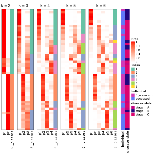
Test correlation between subgroups and known annotations. If the known annotation is numeric, one-way ANOVA test is applied, and if the known annotation is discrete, chi-squared contingency table test is applied.
test_to_known_factors(res)
#> n individual(p) disease.state(p) k
#> ATC:kmeans 54 0.06702 0.761 2
#> ATC:kmeans 28 0.00958 1.000 3
#> ATC:kmeans 49 0.01703 0.544 4
#> ATC:kmeans 39 0.01949 0.429 5
#> ATC:kmeans 48 0.03549 0.270 6
If matrix rows can be associated to genes, consider to use functional_enrichment(res,
...) to perform function enrichment for the signature genes. See this vignette for more detailed explanations.
The object with results only for a single top-value method and a single partition method can be extracted as:
res = res_list["ATC", "skmeans"]
# you can also extract it by
# res = res_list["ATC:skmeans"]
A summary of res and all the functions that can be applied to it:
res
#> A 'ConsensusPartition' object with k = 2, 3, 4, 5, 6.
#> On a matrix with 15834 rows and 54 columns.
#> Top rows (1000, 2000, 3000, 4000, 5000) are extracted by 'ATC' method.
#> Subgroups are detected by 'skmeans' method.
#> Performed in total 1250 partitions by row resampling.
#> Best k for subgroups seems to be 2.
#>
#> Following methods can be applied to this 'ConsensusPartition' object:
#> [1] "cola_report" "collect_classes" "collect_plots"
#> [4] "collect_stats" "colnames" "compare_signatures"
#> [7] "consensus_heatmap" "dimension_reduction" "functional_enrichment"
#> [10] "get_anno_col" "get_anno" "get_classes"
#> [13] "get_consensus" "get_matrix" "get_membership"
#> [16] "get_param" "get_signatures" "get_stats"
#> [19] "is_best_k" "is_stable_k" "membership_heatmap"
#> [22] "ncol" "nrow" "plot_ecdf"
#> [25] "rownames" "select_partition_number" "show"
#> [28] "suggest_best_k" "test_to_known_factors"
collect_plots() function collects all the plots made from res for all k (number of partitions)
into one single page to provide an easy and fast comparison between different k.
collect_plots(res)
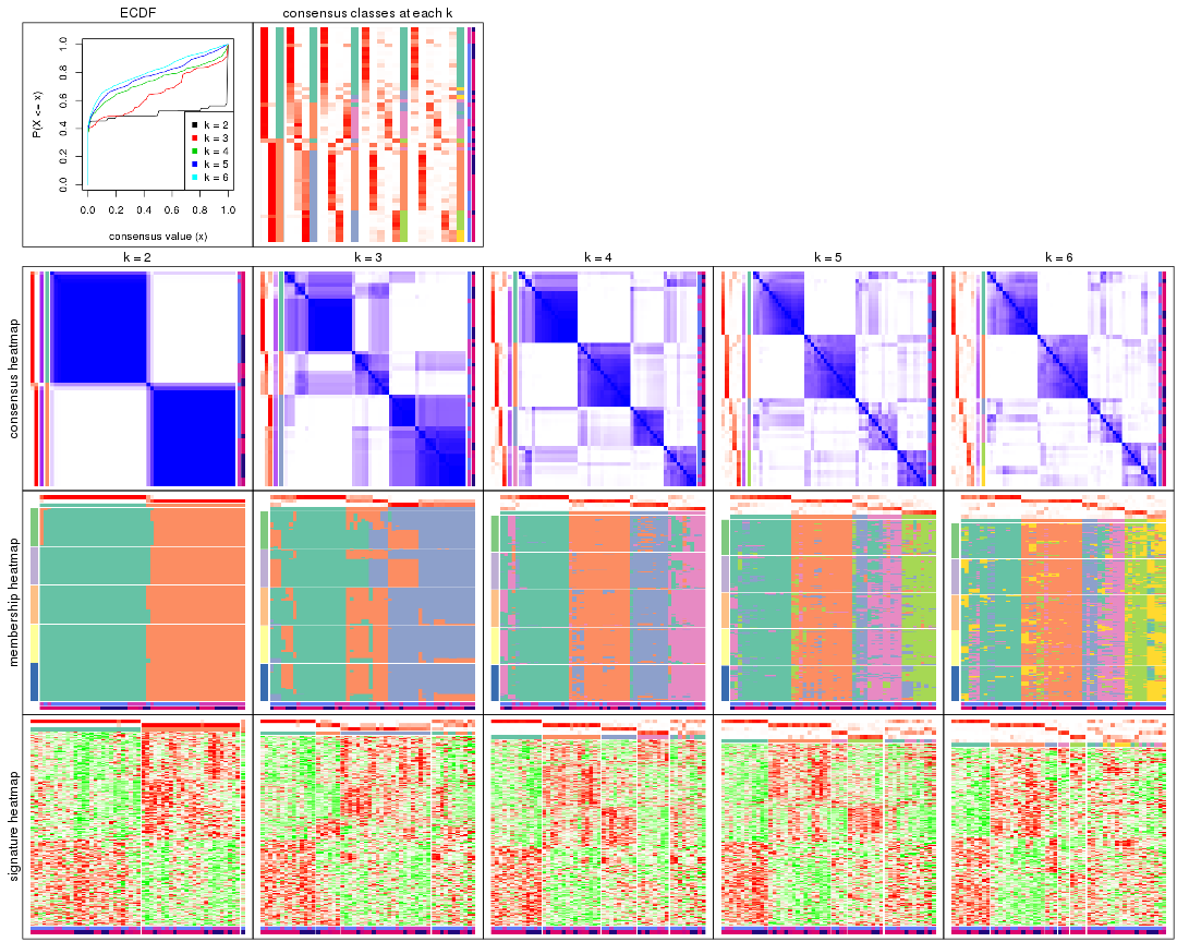
The plots are:
k and the heatmap of
predicted classes for each k.k.k.k.All the plots in panels can be made by individual functions and they are plotted later in this section.
select_partition_number() produces several plots showing different
statistics for choosing “optimized” k. There are following statistics:
k;k, the area increased is defined as \(A_k - A_{k-1}\).The detailed explanations of these statistics can be found in the cola vignette.
Generally speaking, lower PAC score, higher mean silhouette score or higher
concordance corresponds to better partition. Rand index and Jaccard index
measure how similar the current partition is compared to partition with k-1.
If they are too similar, we won't accept k is better than k-1.
select_partition_number(res)
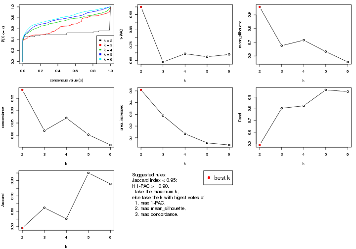
The numeric values for all these statistics can be obtained by get_stats().
get_stats(res)
#> k 1-PAC mean_silhouette concordance area_increased Rand Jaccard
#> 2 2 1.000 0.958 0.984 0.5083 0.491 0.491
#> 3 3 0.640 0.675 0.819 0.2895 0.805 0.623
#> 4 4 0.694 0.715 0.870 0.1339 0.826 0.551
#> 5 5 0.675 0.632 0.803 0.0562 0.962 0.851
#> 6 6 0.689 0.556 0.761 0.0382 0.947 0.778
suggest_best_k() suggests the best \(k\) based on these statistics. The rules are as follows:
suggest_best_k(res)
#> [1] 2
Following shows the table of the partitions (You need to click the show/hide
code output link to see it). The membership matrix (columns with name p*)
is inferred by
clue::cl_consensus()
function with the SE method. Basically the value in the membership matrix
represents the probability to belong to a certain group. The finall class
label for an item is determined with the group with highest probability it
belongs to.
In get_classes() function, the entropy is calculated from the membership
matrix and the silhouette score is calculated from the consensus matrix.
cbind(get_classes(res, k = 2), get_membership(res, k = 2))
#> class entropy silhouette p1 p2
#> GSM311939 2 0.0000 0.9742 0.000 1.000
#> GSM311963 2 0.0000 0.9742 0.000 1.000
#> GSM311973 1 0.0000 0.9919 1.000 0.000
#> GSM311940 2 0.0000 0.9742 0.000 1.000
#> GSM311953 2 0.0000 0.9742 0.000 1.000
#> GSM311974 2 0.0000 0.9742 0.000 1.000
#> GSM311975 2 0.0000 0.9742 0.000 1.000
#> GSM311977 2 0.0000 0.9742 0.000 1.000
#> GSM311982 1 0.0000 0.9919 1.000 0.000
#> GSM311990 2 0.0000 0.9742 0.000 1.000
#> GSM311943 1 0.0000 0.9919 1.000 0.000
#> GSM311944 1 0.0000 0.9919 1.000 0.000
#> GSM311946 2 0.0000 0.9742 0.000 1.000
#> GSM311956 2 0.0000 0.9742 0.000 1.000
#> GSM311967 2 0.0000 0.9742 0.000 1.000
#> GSM311968 2 0.5842 0.8245 0.140 0.860
#> GSM311972 1 0.0000 0.9919 1.000 0.000
#> GSM311980 1 0.0376 0.9884 0.996 0.004
#> GSM311981 1 0.7139 0.7503 0.804 0.196
#> GSM311988 2 0.0000 0.9742 0.000 1.000
#> GSM311957 1 0.0000 0.9919 1.000 0.000
#> GSM311960 2 0.0000 0.9742 0.000 1.000
#> GSM311971 1 0.0000 0.9919 1.000 0.000
#> GSM311976 1 0.0000 0.9919 1.000 0.000
#> GSM311978 1 0.0000 0.9919 1.000 0.000
#> GSM311979 1 0.0000 0.9919 1.000 0.000
#> GSM311983 1 0.0000 0.9919 1.000 0.000
#> GSM311986 2 1.0000 0.0316 0.496 0.504
#> GSM311991 1 0.0000 0.9919 1.000 0.000
#> GSM311938 2 0.0000 0.9742 0.000 1.000
#> GSM311941 2 0.0000 0.9742 0.000 1.000
#> GSM311942 2 0.0000 0.9742 0.000 1.000
#> GSM311945 1 0.0000 0.9919 1.000 0.000
#> GSM311947 2 0.0000 0.9742 0.000 1.000
#> GSM311948 2 0.0000 0.9742 0.000 1.000
#> GSM311949 1 0.0000 0.9919 1.000 0.000
#> GSM311950 2 0.0000 0.9742 0.000 1.000
#> GSM311951 2 0.0000 0.9742 0.000 1.000
#> GSM311952 1 0.0000 0.9919 1.000 0.000
#> GSM311954 2 0.0000 0.9742 0.000 1.000
#> GSM311955 1 0.0000 0.9919 1.000 0.000
#> GSM311958 1 0.0000 0.9919 1.000 0.000
#> GSM311959 1 0.0000 0.9919 1.000 0.000
#> GSM311961 1 0.0000 0.9919 1.000 0.000
#> GSM311962 1 0.0000 0.9919 1.000 0.000
#> GSM311964 1 0.0000 0.9919 1.000 0.000
#> GSM311965 2 0.0000 0.9742 0.000 1.000
#> GSM311966 1 0.0000 0.9919 1.000 0.000
#> GSM311969 1 0.0000 0.9919 1.000 0.000
#> GSM311970 1 0.0938 0.9809 0.988 0.012
#> GSM311984 2 0.0000 0.9742 0.000 1.000
#> GSM311985 1 0.0000 0.9919 1.000 0.000
#> GSM311987 2 0.0000 0.9742 0.000 1.000
#> GSM311989 1 0.0000 0.9919 1.000 0.000
cbind(get_classes(res, k = 3), get_membership(res, k = 3))
#> class entropy silhouette p1 p2 p3
#> GSM311939 3 0.5760 0.828 0.000 0.328 0.672
#> GSM311963 2 0.2959 0.441 0.000 0.900 0.100
#> GSM311973 2 0.5178 0.593 0.256 0.744 0.000
#> GSM311940 3 0.5785 0.827 0.000 0.332 0.668
#> GSM311953 3 0.5785 0.827 0.000 0.332 0.668
#> GSM311974 3 0.5785 0.827 0.000 0.332 0.668
#> GSM311975 3 0.5882 0.816 0.000 0.348 0.652
#> GSM311977 3 0.5926 0.812 0.000 0.356 0.644
#> GSM311982 1 0.0000 0.818 1.000 0.000 0.000
#> GSM311990 3 0.0237 0.727 0.000 0.004 0.996
#> GSM311943 1 0.0237 0.815 0.996 0.000 0.004
#> GSM311944 1 0.0000 0.818 1.000 0.000 0.000
#> GSM311946 3 0.5968 0.805 0.000 0.364 0.636
#> GSM311956 3 0.6291 0.674 0.000 0.468 0.532
#> GSM311967 3 0.5560 0.827 0.000 0.300 0.700
#> GSM311968 3 0.4189 0.598 0.056 0.068 0.876
#> GSM311972 1 0.0000 0.818 1.000 0.000 0.000
#> GSM311980 2 0.0000 0.566 0.000 1.000 0.000
#> GSM311981 2 0.7534 0.185 0.428 0.532 0.040
#> GSM311988 3 0.5785 0.827 0.000 0.332 0.668
#> GSM311957 1 0.6045 0.122 0.620 0.380 0.000
#> GSM311960 2 0.1964 0.505 0.000 0.944 0.056
#> GSM311971 1 0.5785 0.249 0.668 0.332 0.000
#> GSM311976 2 0.6140 0.493 0.404 0.596 0.000
#> GSM311978 1 0.0000 0.818 1.000 0.000 0.000
#> GSM311979 1 0.0000 0.818 1.000 0.000 0.000
#> GSM311983 1 0.0000 0.818 1.000 0.000 0.000
#> GSM311986 1 0.7878 0.338 0.548 0.060 0.392
#> GSM311991 1 0.5098 0.427 0.752 0.248 0.000
#> GSM311938 3 0.5785 0.827 0.000 0.332 0.668
#> GSM311941 3 0.0000 0.726 0.000 0.000 1.000
#> GSM311942 3 0.0000 0.726 0.000 0.000 1.000
#> GSM311945 2 0.6026 0.520 0.376 0.624 0.000
#> GSM311947 3 0.5178 0.818 0.000 0.256 0.744
#> GSM311948 3 0.5254 0.820 0.000 0.264 0.736
#> GSM311949 2 0.6192 0.469 0.420 0.580 0.000
#> GSM311950 3 0.5760 0.828 0.000 0.328 0.672
#> GSM311951 3 0.0237 0.723 0.000 0.004 0.996
#> GSM311952 1 0.0000 0.818 1.000 0.000 0.000
#> GSM311954 3 0.0237 0.728 0.000 0.004 0.996
#> GSM311955 1 0.0237 0.815 0.996 0.000 0.004
#> GSM311958 1 0.0000 0.818 1.000 0.000 0.000
#> GSM311959 1 0.5678 0.494 0.684 0.000 0.316
#> GSM311961 2 0.6410 0.471 0.420 0.576 0.004
#> GSM311962 1 0.0000 0.818 1.000 0.000 0.000
#> GSM311964 2 0.6008 0.532 0.372 0.628 0.000
#> GSM311965 3 0.0000 0.726 0.000 0.000 1.000
#> GSM311966 1 0.0000 0.818 1.000 0.000 0.000
#> GSM311969 1 0.5785 0.477 0.668 0.000 0.332
#> GSM311970 2 0.0000 0.566 0.000 1.000 0.000
#> GSM311984 3 0.5760 0.827 0.000 0.328 0.672
#> GSM311985 1 0.0000 0.818 1.000 0.000 0.000
#> GSM311987 3 0.0000 0.726 0.000 0.000 1.000
#> GSM311989 1 0.4887 0.507 0.772 0.228 0.000
cbind(get_classes(res, k = 4), get_membership(res, k = 4))
#> class entropy silhouette p1 p2 p3 p4
#> GSM311939 2 0.4855 0.4781 0.000 0.644 0.352 0.004
#> GSM311963 2 0.3024 0.8015 0.000 0.852 0.000 0.148
#> GSM311973 4 0.1139 0.7752 0.012 0.008 0.008 0.972
#> GSM311940 2 0.0188 0.9016 0.000 0.996 0.000 0.004
#> GSM311953 2 0.0188 0.9016 0.000 0.996 0.000 0.004
#> GSM311974 2 0.1545 0.8928 0.000 0.952 0.040 0.008
#> GSM311975 2 0.1174 0.8955 0.000 0.968 0.020 0.012
#> GSM311977 2 0.0336 0.9010 0.000 0.992 0.000 0.008
#> GSM311982 1 0.0188 0.8308 0.996 0.000 0.000 0.004
#> GSM311990 3 0.2647 0.8373 0.000 0.120 0.880 0.000
#> GSM311943 1 0.0469 0.8266 0.988 0.000 0.012 0.000
#> GSM311944 1 0.0336 0.8283 0.992 0.000 0.008 0.000
#> GSM311946 2 0.0592 0.8997 0.000 0.984 0.000 0.016
#> GSM311956 2 0.1211 0.8863 0.000 0.960 0.000 0.040
#> GSM311967 2 0.0592 0.9009 0.000 0.984 0.016 0.000
#> GSM311968 3 0.1007 0.8240 0.008 0.008 0.976 0.008
#> GSM311972 1 0.0937 0.8196 0.976 0.000 0.012 0.012
#> GSM311980 4 0.1042 0.7694 0.000 0.020 0.008 0.972
#> GSM311981 1 0.8175 -0.0181 0.412 0.200 0.020 0.368
#> GSM311988 2 0.1970 0.8858 0.000 0.932 0.060 0.008
#> GSM311957 4 0.6090 0.4384 0.384 0.000 0.052 0.564
#> GSM311960 4 0.5346 0.6251 0.000 0.192 0.076 0.732
#> GSM311971 1 0.4989 -0.2019 0.528 0.000 0.000 0.472
#> GSM311976 4 0.4252 0.6829 0.252 0.000 0.004 0.744
#> GSM311978 1 0.0188 0.8308 0.996 0.000 0.000 0.004
#> GSM311979 1 0.0188 0.8308 0.996 0.000 0.000 0.004
#> GSM311983 1 0.0188 0.8308 0.996 0.000 0.000 0.004
#> GSM311986 3 0.2048 0.7938 0.064 0.000 0.928 0.008
#> GSM311991 1 0.4999 0.4132 0.660 0.000 0.012 0.328
#> GSM311938 2 0.0188 0.9017 0.000 0.996 0.004 0.000
#> GSM311941 3 0.1557 0.8459 0.000 0.056 0.944 0.000
#> GSM311942 3 0.0707 0.8330 0.000 0.020 0.980 0.000
#> GSM311945 4 0.3919 0.7625 0.104 0.000 0.056 0.840
#> GSM311947 2 0.3528 0.7623 0.000 0.808 0.192 0.000
#> GSM311948 2 0.4608 0.5875 0.000 0.692 0.304 0.004
#> GSM311949 4 0.4560 0.6341 0.296 0.000 0.004 0.700
#> GSM311950 2 0.2197 0.8720 0.000 0.916 0.080 0.004
#> GSM311951 3 0.2408 0.8266 0.000 0.104 0.896 0.000
#> GSM311952 1 0.0376 0.8302 0.992 0.000 0.004 0.004
#> GSM311954 3 0.3402 0.8027 0.000 0.164 0.832 0.004
#> GSM311955 1 0.0592 0.8244 0.984 0.000 0.016 0.000
#> GSM311958 1 0.0000 0.8301 1.000 0.000 0.000 0.000
#> GSM311959 1 0.4608 0.4762 0.692 0.004 0.304 0.000
#> GSM311961 4 0.6810 0.4427 0.292 0.088 0.016 0.604
#> GSM311962 1 0.0188 0.8308 0.996 0.000 0.000 0.004
#> GSM311964 4 0.2342 0.7680 0.080 0.000 0.008 0.912
#> GSM311965 3 0.3052 0.8260 0.000 0.136 0.860 0.004
#> GSM311966 1 0.0188 0.8308 0.996 0.000 0.000 0.004
#> GSM311969 3 0.5336 -0.0851 0.496 0.004 0.496 0.004
#> GSM311970 4 0.0592 0.7696 0.000 0.016 0.000 0.984
#> GSM311984 2 0.1109 0.8965 0.000 0.968 0.028 0.004
#> GSM311985 1 0.1059 0.8171 0.972 0.000 0.012 0.016
#> GSM311987 3 0.3074 0.8169 0.000 0.152 0.848 0.000
#> GSM311989 1 0.5977 -0.1534 0.528 0.000 0.040 0.432
cbind(get_classes(res, k = 5), get_membership(res, k = 5))
#> class entropy silhouette p1 p2 p3 p4 p5
#> GSM311939 2 0.4173 0.5745 0.000 0.688 0.012 0.000 0.300
#> GSM311963 2 0.4161 0.6082 0.000 0.704 0.016 0.280 0.000
#> GSM311973 4 0.1300 0.5810 0.016 0.000 0.028 0.956 0.000
#> GSM311940 2 0.0290 0.8667 0.000 0.992 0.008 0.000 0.000
#> GSM311953 2 0.0324 0.8657 0.000 0.992 0.004 0.004 0.000
#> GSM311974 2 0.0833 0.8660 0.000 0.976 0.004 0.004 0.016
#> GSM311975 2 0.3992 0.7094 0.000 0.720 0.268 0.000 0.012
#> GSM311977 2 0.0693 0.8662 0.000 0.980 0.012 0.008 0.000
#> GSM311982 1 0.1310 0.7692 0.956 0.000 0.020 0.024 0.000
#> GSM311990 5 0.3704 0.7750 0.000 0.088 0.092 0.000 0.820
#> GSM311943 1 0.2629 0.7284 0.880 0.000 0.104 0.004 0.012
#> GSM311944 1 0.1608 0.7586 0.928 0.000 0.072 0.000 0.000
#> GSM311946 2 0.0865 0.8641 0.000 0.972 0.004 0.024 0.000
#> GSM311956 2 0.1877 0.8460 0.000 0.924 0.064 0.012 0.000
#> GSM311967 2 0.2660 0.8249 0.000 0.864 0.128 0.000 0.008
#> GSM311968 5 0.2619 0.7394 0.004 0.004 0.024 0.072 0.896
#> GSM311972 1 0.3876 0.4458 0.684 0.000 0.316 0.000 0.000
#> GSM311980 4 0.2006 0.5534 0.000 0.012 0.072 0.916 0.000
#> GSM311981 3 0.4784 0.3794 0.032 0.068 0.764 0.136 0.000
#> GSM311988 2 0.1329 0.8630 0.000 0.956 0.008 0.004 0.032
#> GSM311957 4 0.6035 0.3826 0.376 0.000 0.020 0.532 0.072
#> GSM311960 4 0.4639 0.5047 0.000 0.104 0.024 0.776 0.096
#> GSM311971 1 0.4624 0.2333 0.636 0.000 0.024 0.340 0.000
#> GSM311976 4 0.5769 0.4443 0.340 0.000 0.104 0.556 0.000
#> GSM311978 1 0.0451 0.7782 0.988 0.000 0.008 0.004 0.000
#> GSM311979 1 0.1310 0.7692 0.956 0.000 0.020 0.024 0.000
#> GSM311983 1 0.0162 0.7790 0.996 0.000 0.000 0.004 0.000
#> GSM311986 5 0.4461 0.6916 0.064 0.000 0.080 0.056 0.800
#> GSM311991 3 0.5888 0.3608 0.316 0.000 0.560 0.124 0.000
#> GSM311938 2 0.1082 0.8639 0.000 0.964 0.028 0.000 0.008
#> GSM311941 5 0.1740 0.7872 0.000 0.012 0.056 0.000 0.932
#> GSM311942 5 0.0613 0.7744 0.000 0.004 0.004 0.008 0.984
#> GSM311945 4 0.4666 0.5619 0.080 0.000 0.036 0.780 0.104
#> GSM311947 2 0.4216 0.7578 0.000 0.780 0.120 0.000 0.100
#> GSM311948 2 0.4382 0.6167 0.000 0.700 0.020 0.004 0.276
#> GSM311949 4 0.5641 0.4383 0.356 0.000 0.088 0.556 0.000
#> GSM311950 2 0.1992 0.8565 0.000 0.924 0.032 0.000 0.044
#> GSM311951 5 0.2930 0.7526 0.000 0.076 0.032 0.012 0.880
#> GSM311952 1 0.1197 0.7700 0.952 0.000 0.048 0.000 0.000
#> GSM311954 5 0.5758 0.6498 0.000 0.124 0.284 0.000 0.592
#> GSM311955 1 0.3556 0.6657 0.808 0.000 0.168 0.004 0.020
#> GSM311958 1 0.0609 0.7768 0.980 0.000 0.020 0.000 0.000
#> GSM311959 1 0.6386 0.1062 0.508 0.000 0.324 0.004 0.164
#> GSM311961 3 0.5979 0.3209 0.132 0.020 0.636 0.212 0.000
#> GSM311962 1 0.1018 0.7757 0.968 0.000 0.016 0.016 0.000
#> GSM311964 4 0.5828 0.2160 0.100 0.000 0.380 0.520 0.000
#> GSM311965 5 0.4948 0.7179 0.000 0.068 0.256 0.000 0.676
#> GSM311966 1 0.0798 0.7765 0.976 0.000 0.016 0.008 0.000
#> GSM311969 3 0.6933 -0.0508 0.316 0.000 0.376 0.004 0.304
#> GSM311970 4 0.3671 0.4266 0.000 0.008 0.236 0.756 0.000
#> GSM311984 2 0.2873 0.8318 0.000 0.860 0.120 0.000 0.020
#> GSM311985 1 0.3636 0.5282 0.728 0.000 0.272 0.000 0.000
#> GSM311987 5 0.5258 0.7129 0.000 0.104 0.232 0.000 0.664
#> GSM311989 1 0.6093 0.0471 0.552 0.000 0.024 0.348 0.076
cbind(get_classes(res, k = 6), get_membership(res, k = 6))
#> class entropy silhouette p1 p2 p3 p4 p5 p6
#> GSM311939 2 0.5072 0.491 0.000 0.600 0.004 0.012 0.328 0.056
#> GSM311963 2 0.4624 0.453 0.000 0.592 0.008 0.372 0.004 0.024
#> GSM311973 4 0.1413 0.551 0.004 0.000 0.036 0.948 0.004 0.008
#> GSM311940 2 0.0146 0.814 0.000 0.996 0.004 0.000 0.000 0.000
#> GSM311953 2 0.0692 0.814 0.000 0.976 0.000 0.020 0.000 0.004
#> GSM311974 2 0.2102 0.810 0.000 0.920 0.004 0.024 0.032 0.020
#> GSM311975 2 0.5123 0.568 0.000 0.628 0.188 0.000 0.000 0.184
#> GSM311977 2 0.0508 0.815 0.000 0.984 0.004 0.012 0.000 0.000
#> GSM311982 1 0.1350 0.728 0.952 0.000 0.020 0.008 0.000 0.020
#> GSM311990 5 0.4549 0.457 0.000 0.068 0.008 0.000 0.692 0.232
#> GSM311943 1 0.3834 0.567 0.708 0.000 0.024 0.000 0.000 0.268
#> GSM311944 1 0.2278 0.707 0.868 0.000 0.004 0.000 0.000 0.128
#> GSM311946 2 0.1461 0.813 0.000 0.940 0.000 0.044 0.000 0.016
#> GSM311956 2 0.1930 0.806 0.000 0.916 0.036 0.048 0.000 0.000
#> GSM311967 2 0.3176 0.745 0.000 0.812 0.032 0.000 0.000 0.156
#> GSM311968 5 0.2177 0.679 0.000 0.000 0.008 0.032 0.908 0.052
#> GSM311972 1 0.4889 0.129 0.504 0.000 0.436 0.000 0.000 0.060
#> GSM311980 4 0.1701 0.523 0.000 0.008 0.072 0.920 0.000 0.000
#> GSM311981 3 0.3386 0.671 0.028 0.036 0.856 0.028 0.000 0.052
#> GSM311988 2 0.3007 0.792 0.000 0.864 0.004 0.020 0.080 0.032
#> GSM311957 4 0.7252 0.191 0.384 0.000 0.052 0.396 0.064 0.104
#> GSM311960 4 0.4897 0.501 0.000 0.068 0.040 0.760 0.076 0.056
#> GSM311971 1 0.4921 0.410 0.688 0.000 0.036 0.212 0.000 0.064
#> GSM311976 4 0.6496 0.269 0.372 0.000 0.124 0.440 0.000 0.064
#> GSM311978 1 0.0622 0.742 0.980 0.000 0.008 0.000 0.000 0.012
#> GSM311979 1 0.1515 0.724 0.944 0.000 0.020 0.008 0.000 0.028
#> GSM311983 1 0.0603 0.742 0.980 0.000 0.004 0.000 0.000 0.016
#> GSM311986 5 0.4970 0.429 0.032 0.000 0.012 0.020 0.636 0.300
#> GSM311991 3 0.3098 0.655 0.164 0.000 0.812 0.024 0.000 0.000
#> GSM311938 2 0.1320 0.807 0.000 0.948 0.016 0.000 0.000 0.036
#> GSM311941 5 0.3030 0.648 0.000 0.008 0.008 0.000 0.816 0.168
#> GSM311942 5 0.1141 0.708 0.000 0.000 0.000 0.000 0.948 0.052
#> GSM311945 4 0.6204 0.498 0.092 0.000 0.088 0.660 0.084 0.076
#> GSM311947 2 0.4162 0.715 0.000 0.760 0.028 0.000 0.044 0.168
#> GSM311948 2 0.4892 0.574 0.000 0.644 0.008 0.004 0.280 0.064
#> GSM311949 1 0.6349 -0.260 0.432 0.000 0.120 0.396 0.000 0.052
#> GSM311950 2 0.2862 0.799 0.000 0.864 0.008 0.000 0.048 0.080
#> GSM311951 5 0.3351 0.654 0.000 0.040 0.020 0.000 0.832 0.108
#> GSM311952 1 0.2250 0.724 0.888 0.000 0.020 0.000 0.000 0.092
#> GSM311954 6 0.5838 0.351 0.000 0.092 0.048 0.000 0.292 0.568
#> GSM311955 1 0.4530 0.407 0.600 0.000 0.044 0.000 0.000 0.356
#> GSM311958 1 0.1391 0.740 0.944 0.000 0.016 0.000 0.000 0.040
#> GSM311959 6 0.5293 0.306 0.292 0.000 0.036 0.000 0.060 0.612
#> GSM311961 3 0.3544 0.676 0.036 0.008 0.840 0.056 0.000 0.060
#> GSM311962 1 0.1194 0.734 0.956 0.000 0.004 0.008 0.000 0.032
#> GSM311964 3 0.5708 0.152 0.080 0.000 0.512 0.376 0.000 0.032
#> GSM311965 6 0.5668 0.157 0.000 0.048 0.052 0.000 0.416 0.484
#> GSM311966 1 0.0260 0.741 0.992 0.000 0.008 0.000 0.000 0.000
#> GSM311969 6 0.5539 0.391 0.172 0.000 0.076 0.000 0.092 0.660
#> GSM311970 4 0.3104 0.380 0.000 0.004 0.204 0.788 0.000 0.004
#> GSM311984 2 0.5114 0.652 0.000 0.696 0.108 0.000 0.044 0.152
#> GSM311985 1 0.4587 0.327 0.596 0.000 0.356 0.000 0.000 0.048
#> GSM311987 6 0.5486 0.291 0.000 0.088 0.020 0.000 0.332 0.560
#> GSM311989 1 0.6806 0.230 0.564 0.000 0.048 0.216 0.072 0.100
Heatmaps for the consensus matrix. It visualizes the probability of two samples to be in a same group.
consensus_heatmap(res, k = 2)
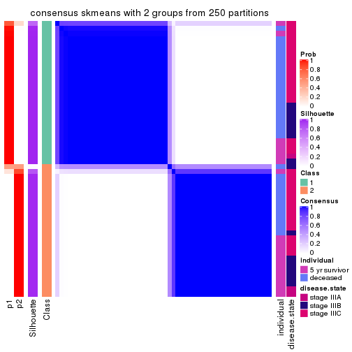
consensus_heatmap(res, k = 3)
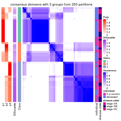
consensus_heatmap(res, k = 4)
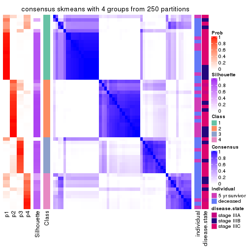
consensus_heatmap(res, k = 5)
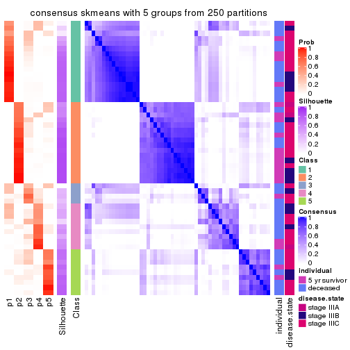
consensus_heatmap(res, k = 6)
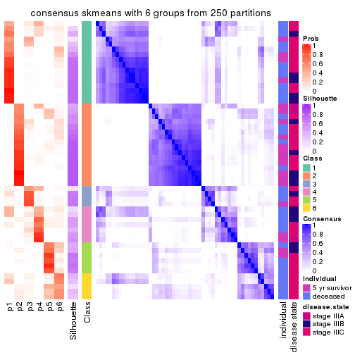
Heatmaps for the membership of samples in all partitions to see how consistent they are:
membership_heatmap(res, k = 2)
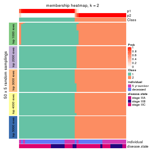
membership_heatmap(res, k = 3)
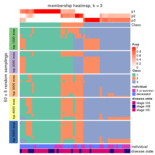
membership_heatmap(res, k = 4)
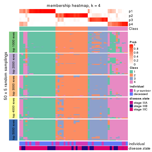
membership_heatmap(res, k = 5)
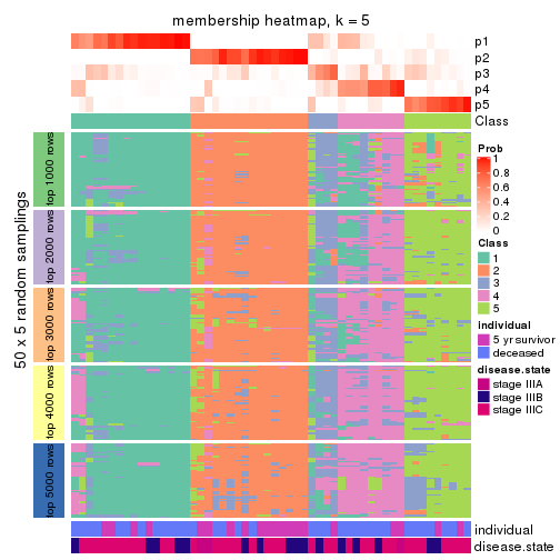
membership_heatmap(res, k = 6)
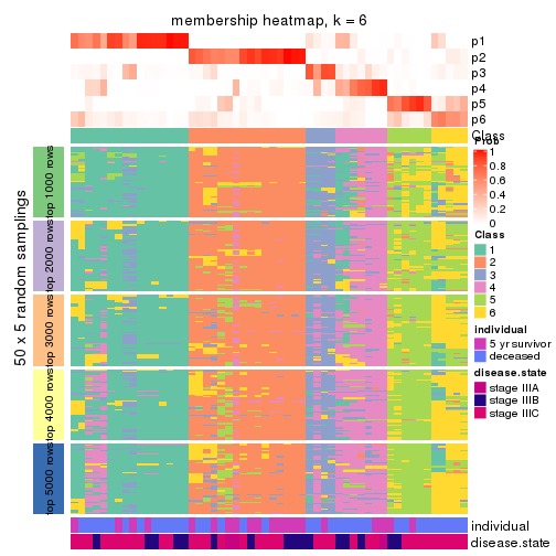
As soon as we have had the classes for columns, we can look for signatures which are significantly different between classes which can be candidate marks for certain classes. Following are the heatmaps for signatures.
Signature heatmaps where rows are scaled:
get_signatures(res, k = 2)
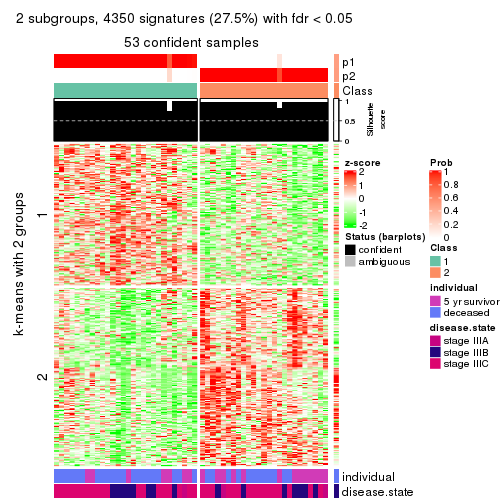
get_signatures(res, k = 3)
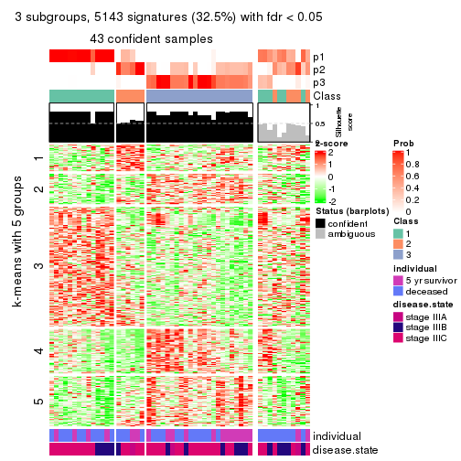
get_signatures(res, k = 4)
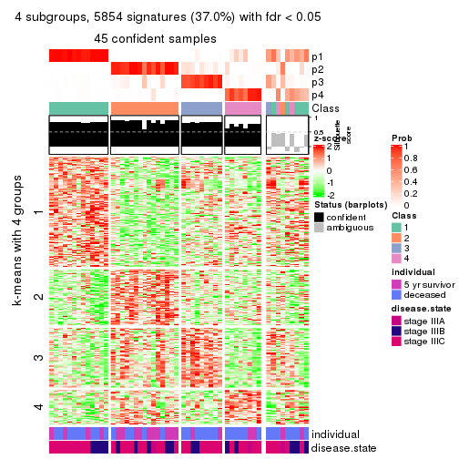
get_signatures(res, k = 5)
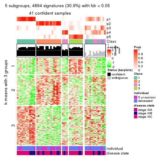
get_signatures(res, k = 6)
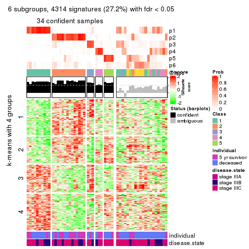
Signature heatmaps where rows are not scaled:
get_signatures(res, k = 2, scale_rows = FALSE)
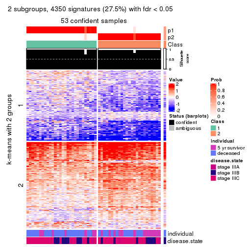
get_signatures(res, k = 3, scale_rows = FALSE)
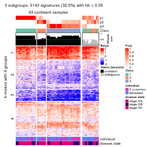
get_signatures(res, k = 4, scale_rows = FALSE)
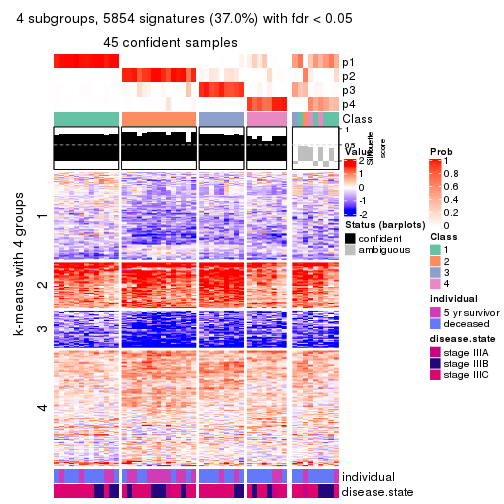
get_signatures(res, k = 5, scale_rows = FALSE)
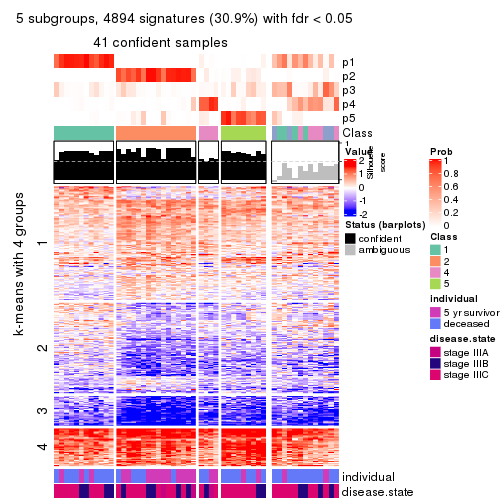
get_signatures(res, k = 6, scale_rows = FALSE)
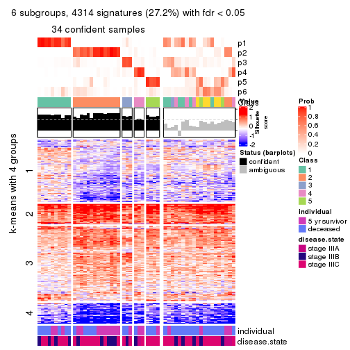
Compare the overlap of signatures from different k:
compare_signatures(res)
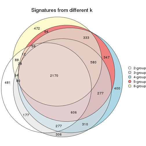
get_signature() returns a data frame invisibly. TO get the list of signatures, the function
call should be assigned to a variable explicitly. In following code, if plot argument is set
to FALSE, no heatmap is plotted while only the differential analysis is performed.
# code only for demonstration
tb = get_signature(res, k = ..., plot = FALSE)
An example of the output of tb is:
#> which_row fdr mean_1 mean_2 scaled_mean_1 scaled_mean_2 km
#> 1 38 0.042760348 8.373488 9.131774 -0.5533452 0.5164555 1
#> 2 40 0.018707592 7.106213 8.469186 -0.6173731 0.5762149 1
#> 3 55 0.019134737 10.221463 11.207825 -0.6159697 0.5749050 1
#> 4 59 0.006059896 5.921854 7.869574 -0.6899429 0.6439467 1
#> 5 60 0.018055526 8.928898 10.211722 -0.6204761 0.5791110 1
#> 6 98 0.009384629 15.714769 14.887706 0.6635654 -0.6193277 2
...
The columns in tb are:
which_row: row indices corresponding to the input matrix.fdr: FDR for the differential test. mean_x: The mean value in group x.scaled_mean_x: The mean value in group x after rows are scaled.km: Row groups if k-means clustering is applied to rows.UMAP plot which shows how samples are separated.
dimension_reduction(res, k = 2, method = "UMAP")
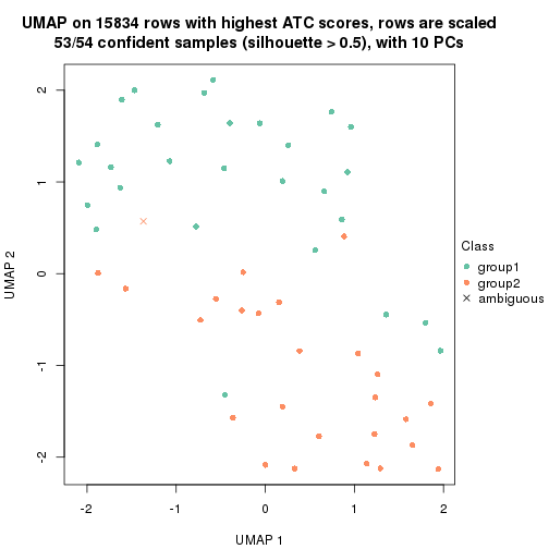
dimension_reduction(res, k = 3, method = "UMAP")
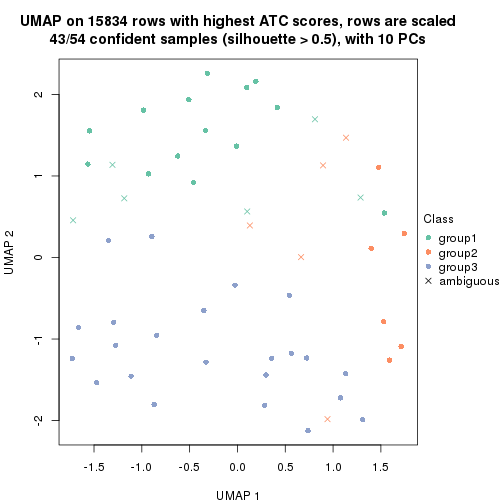
dimension_reduction(res, k = 4, method = "UMAP")
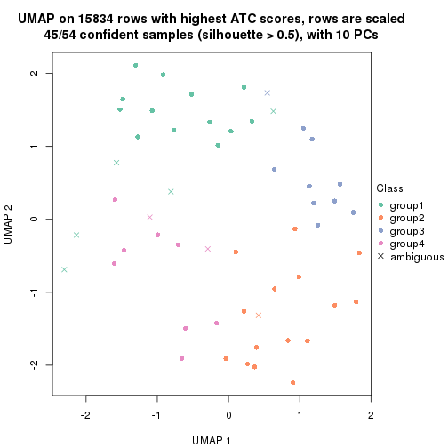
dimension_reduction(res, k = 5, method = "UMAP")
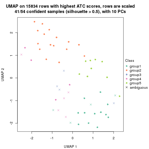
dimension_reduction(res, k = 6, method = "UMAP")
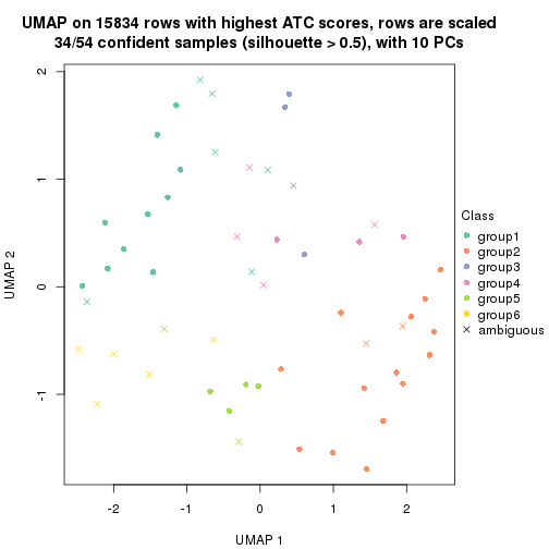
Following heatmap shows how subgroups are split when increasing k:
collect_classes(res)
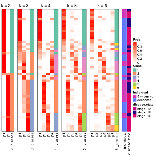
Test correlation between subgroups and known annotations. If the known annotation is numeric, one-way ANOVA test is applied, and if the known annotation is discrete, chi-squared contingency table test is applied.
test_to_known_factors(res)
#> n individual(p) disease.state(p) k
#> ATC:skmeans 53 0.0818 0.783 2
#> ATC:skmeans 43 0.3328 0.597 3
#> ATC:skmeans 45 0.0771 0.820 4
#> ATC:skmeans 41 0.0568 0.589 5
#> ATC:skmeans 34 0.3661 0.108 6
If matrix rows can be associated to genes, consider to use functional_enrichment(res,
...) to perform function enrichment for the signature genes. See this vignette for more detailed explanations.
The object with results only for a single top-value method and a single partition method can be extracted as:
res = res_list["ATC", "pam"]
# you can also extract it by
# res = res_list["ATC:pam"]
A summary of res and all the functions that can be applied to it:
res
#> A 'ConsensusPartition' object with k = 2, 3, 4, 5, 6.
#> On a matrix with 15834 rows and 54 columns.
#> Top rows (1000, 2000, 3000, 4000, 5000) are extracted by 'ATC' method.
#> Subgroups are detected by 'pam' method.
#> Performed in total 1250 partitions by row resampling.
#> Best k for subgroups seems to be 2.
#>
#> Following methods can be applied to this 'ConsensusPartition' object:
#> [1] "cola_report" "collect_classes" "collect_plots"
#> [4] "collect_stats" "colnames" "compare_signatures"
#> [7] "consensus_heatmap" "dimension_reduction" "functional_enrichment"
#> [10] "get_anno_col" "get_anno" "get_classes"
#> [13] "get_consensus" "get_matrix" "get_membership"
#> [16] "get_param" "get_signatures" "get_stats"
#> [19] "is_best_k" "is_stable_k" "membership_heatmap"
#> [22] "ncol" "nrow" "plot_ecdf"
#> [25] "rownames" "select_partition_number" "show"
#> [28] "suggest_best_k" "test_to_known_factors"
collect_plots() function collects all the plots made from res for all k (number of partitions)
into one single page to provide an easy and fast comparison between different k.
collect_plots(res)
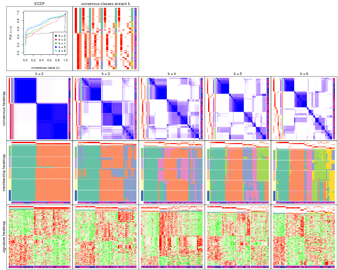
The plots are:
k and the heatmap of
predicted classes for each k.k.k.k.All the plots in panels can be made by individual functions and they are plotted later in this section.
select_partition_number() produces several plots showing different
statistics for choosing “optimized” k. There are following statistics:
k;k, the area increased is defined as \(A_k - A_{k-1}\).The detailed explanations of these statistics can be found in the cola vignette.
Generally speaking, lower PAC score, higher mean silhouette score or higher
concordance corresponds to better partition. Rand index and Jaccard index
measure how similar the current partition is compared to partition with k-1.
If they are too similar, we won't accept k is better than k-1.
select_partition_number(res)
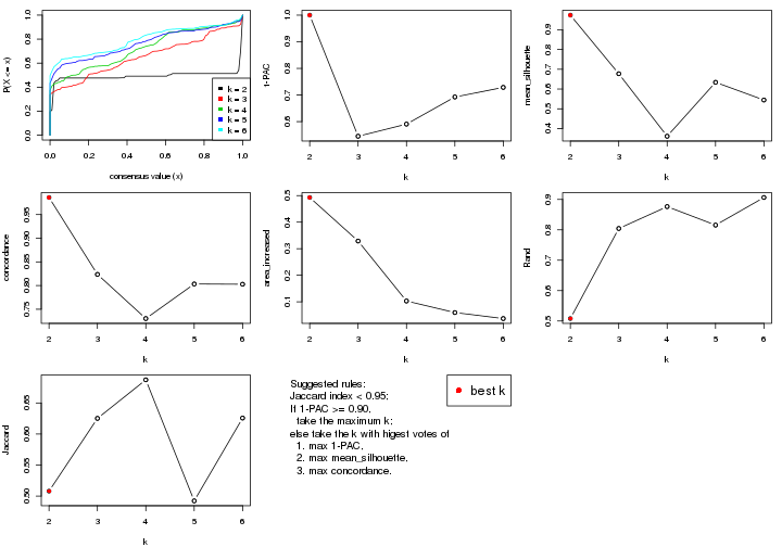
The numeric values for all these statistics can be obtained by get_stats().
get_stats(res)
#> k 1-PAC mean_silhouette concordance area_increased Rand Jaccard
#> 2 2 1.000 0.974 0.986 0.4930 0.508 0.508
#> 3 3 0.545 0.677 0.824 0.3290 0.804 0.625
#> 4 4 0.591 0.361 0.730 0.1031 0.876 0.687
#> 5 5 0.693 0.634 0.803 0.0596 0.816 0.492
#> 6 6 0.729 0.544 0.803 0.0370 0.906 0.626
suggest_best_k() suggests the best \(k\) based on these statistics. The rules are as follows:
suggest_best_k(res)
#> [1] 2
Following shows the table of the partitions (You need to click the show/hide
code output link to see it). The membership matrix (columns with name p*)
is inferred by
clue::cl_consensus()
function with the SE method. Basically the value in the membership matrix
represents the probability to belong to a certain group. The finall class
label for an item is determined with the group with highest probability it
belongs to.
In get_classes() function, the entropy is calculated from the membership
matrix and the silhouette score is calculated from the consensus matrix.
cbind(get_classes(res, k = 2), get_membership(res, k = 2))
#> class entropy silhouette p1 p2
#> GSM311939 2 0.0672 0.978 0.008 0.992
#> GSM311963 2 0.0938 0.978 0.012 0.988
#> GSM311973 2 0.1414 0.978 0.020 0.980
#> GSM311940 2 0.0000 0.978 0.000 1.000
#> GSM311953 2 0.0000 0.978 0.000 1.000
#> GSM311974 2 0.0000 0.978 0.000 1.000
#> GSM311975 2 0.0000 0.978 0.000 1.000
#> GSM311977 2 0.0000 0.978 0.000 1.000
#> GSM311982 1 0.0000 0.997 1.000 0.000
#> GSM311990 2 0.0000 0.978 0.000 1.000
#> GSM311943 1 0.0000 0.997 1.000 0.000
#> GSM311944 1 0.0000 0.997 1.000 0.000
#> GSM311946 2 0.1414 0.978 0.020 0.980
#> GSM311956 2 0.0000 0.978 0.000 1.000
#> GSM311967 2 0.0000 0.978 0.000 1.000
#> GSM311968 2 0.1414 0.978 0.020 0.980
#> GSM311972 1 0.0000 0.997 1.000 0.000
#> GSM311980 2 0.1414 0.978 0.020 0.980
#> GSM311981 2 0.1414 0.978 0.020 0.980
#> GSM311988 2 0.0000 0.978 0.000 1.000
#> GSM311957 1 0.0000 0.997 1.000 0.000
#> GSM311960 2 0.1414 0.978 0.020 0.980
#> GSM311971 1 0.0000 0.997 1.000 0.000
#> GSM311976 1 0.0000 0.997 1.000 0.000
#> GSM311978 1 0.0000 0.997 1.000 0.000
#> GSM311979 1 0.0000 0.997 1.000 0.000
#> GSM311983 1 0.0000 0.997 1.000 0.000
#> GSM311986 1 0.1843 0.971 0.972 0.028
#> GSM311991 1 0.0000 0.997 1.000 0.000
#> GSM311938 2 0.0000 0.978 0.000 1.000
#> GSM311941 2 0.1414 0.978 0.020 0.980
#> GSM311942 2 0.1414 0.978 0.020 0.980
#> GSM311945 2 0.1414 0.978 0.020 0.980
#> GSM311947 2 0.0000 0.978 0.000 1.000
#> GSM311948 2 0.1414 0.978 0.020 0.980
#> GSM311949 1 0.0000 0.997 1.000 0.000
#> GSM311950 2 0.0000 0.978 0.000 1.000
#> GSM311951 2 0.1414 0.978 0.020 0.980
#> GSM311952 1 0.0000 0.997 1.000 0.000
#> GSM311954 2 0.0938 0.978 0.012 0.988
#> GSM311955 1 0.0000 0.997 1.000 0.000
#> GSM311958 1 0.0000 0.997 1.000 0.000
#> GSM311959 1 0.0000 0.997 1.000 0.000
#> GSM311961 2 0.1414 0.978 0.020 0.980
#> GSM311962 1 0.0000 0.997 1.000 0.000
#> GSM311964 2 0.9635 0.392 0.388 0.612
#> GSM311965 2 0.1414 0.978 0.020 0.980
#> GSM311966 1 0.0000 0.997 1.000 0.000
#> GSM311969 1 0.1633 0.975 0.976 0.024
#> GSM311970 2 0.1414 0.978 0.020 0.980
#> GSM311984 2 0.0000 0.978 0.000 1.000
#> GSM311985 1 0.0000 0.997 1.000 0.000
#> GSM311987 2 0.0000 0.978 0.000 1.000
#> GSM311989 1 0.0000 0.997 1.000 0.000
cbind(get_classes(res, k = 3), get_membership(res, k = 3))
#> class entropy silhouette p1 p2 p3
#> GSM311939 2 0.5254 0.6821 0.000 0.736 0.264
#> GSM311963 2 0.3340 0.7870 0.000 0.880 0.120
#> GSM311973 2 0.0592 0.7705 0.000 0.988 0.012
#> GSM311940 2 0.4291 0.7813 0.000 0.820 0.180
#> GSM311953 2 0.4291 0.7813 0.000 0.820 0.180
#> GSM311974 2 0.4291 0.7813 0.000 0.820 0.180
#> GSM311975 2 0.4291 0.7813 0.000 0.820 0.180
#> GSM311977 2 0.4291 0.7813 0.000 0.820 0.180
#> GSM311982 1 0.0000 0.8534 1.000 0.000 0.000
#> GSM311990 3 0.4504 0.5929 0.000 0.196 0.804
#> GSM311943 1 0.9231 0.4196 0.512 0.180 0.308
#> GSM311944 1 0.2625 0.8173 0.916 0.000 0.084
#> GSM311946 2 0.0237 0.7785 0.000 0.996 0.004
#> GSM311956 2 0.4291 0.7813 0.000 0.820 0.180
#> GSM311967 3 0.5859 0.4317 0.000 0.344 0.656
#> GSM311968 3 0.6235 0.4549 0.000 0.436 0.564
#> GSM311972 1 0.0000 0.8534 1.000 0.000 0.000
#> GSM311980 2 0.0000 0.7775 0.000 1.000 0.000
#> GSM311981 2 0.5926 0.0905 0.000 0.644 0.356
#> GSM311988 2 0.4291 0.7813 0.000 0.820 0.180
#> GSM311957 1 0.5277 0.7188 0.796 0.180 0.024
#> GSM311960 2 0.0592 0.7705 0.000 0.988 0.012
#> GSM311971 1 0.0000 0.8534 1.000 0.000 0.000
#> GSM311976 1 0.0424 0.8505 0.992 0.008 0.000
#> GSM311978 1 0.0000 0.8534 1.000 0.000 0.000
#> GSM311979 1 0.0000 0.8534 1.000 0.000 0.000
#> GSM311983 1 0.0000 0.8534 1.000 0.000 0.000
#> GSM311986 3 0.7815 0.4572 0.148 0.180 0.672
#> GSM311991 1 0.0000 0.8534 1.000 0.000 0.000
#> GSM311938 2 0.4291 0.7813 0.000 0.820 0.180
#> GSM311941 3 0.5529 0.6260 0.000 0.296 0.704
#> GSM311942 3 0.4931 0.6015 0.000 0.232 0.768
#> GSM311945 2 0.0892 0.7635 0.000 0.980 0.020
#> GSM311947 3 0.5905 0.4161 0.000 0.352 0.648
#> GSM311948 2 0.0000 0.7775 0.000 1.000 0.000
#> GSM311949 1 0.4700 0.7263 0.812 0.180 0.008
#> GSM311950 3 0.6168 0.2755 0.000 0.412 0.588
#> GSM311951 2 0.0592 0.7705 0.000 0.988 0.012
#> GSM311952 1 0.8396 0.5922 0.624 0.180 0.196
#> GSM311954 3 0.1411 0.6267 0.000 0.036 0.964
#> GSM311955 1 0.5327 0.6707 0.728 0.000 0.272
#> GSM311958 1 0.0000 0.8534 1.000 0.000 0.000
#> GSM311959 3 0.6307 0.1446 0.328 0.012 0.660
#> GSM311961 2 0.0747 0.7674 0.000 0.984 0.016
#> GSM311962 1 0.0000 0.8534 1.000 0.000 0.000
#> GSM311964 2 0.6490 0.1960 0.360 0.628 0.012
#> GSM311965 3 0.5926 0.6030 0.000 0.356 0.644
#> GSM311966 1 0.0000 0.8534 1.000 0.000 0.000
#> GSM311969 1 0.7581 0.3211 0.496 0.040 0.464
#> GSM311970 2 0.0000 0.7775 0.000 1.000 0.000
#> GSM311984 2 0.4291 0.7813 0.000 0.820 0.180
#> GSM311985 1 0.3686 0.7453 0.860 0.000 0.140
#> GSM311987 3 0.4504 0.5929 0.000 0.196 0.804
#> GSM311989 1 0.8026 0.6248 0.656 0.180 0.164
cbind(get_classes(res, k = 4), get_membership(res, k = 4))
#> class entropy silhouette p1 p2 p3 p4
#> GSM311939 2 0.4898 0.2696 0.000 0.584 0.416 0.000
#> GSM311963 2 0.0188 0.6096 0.000 0.996 0.004 0.000
#> GSM311973 2 0.5105 0.5214 0.432 0.564 0.004 0.000
#> GSM311940 2 0.4040 0.4525 0.000 0.752 0.000 0.248
#> GSM311953 2 0.3219 0.5231 0.000 0.836 0.000 0.164
#> GSM311974 2 0.0707 0.6034 0.000 0.980 0.000 0.020
#> GSM311975 2 0.4991 0.3143 0.000 0.608 0.388 0.004
#> GSM311977 2 0.0188 0.6096 0.000 0.996 0.004 0.000
#> GSM311982 1 0.4933 0.2846 0.568 0.000 0.000 0.432
#> GSM311990 3 0.3219 0.6008 0.000 0.164 0.836 0.000
#> GSM311943 1 0.3444 0.1936 0.816 0.000 0.184 0.000
#> GSM311944 1 0.6546 0.1729 0.492 0.000 0.076 0.432
#> GSM311946 2 0.0188 0.6096 0.000 0.996 0.004 0.000
#> GSM311956 2 0.0188 0.6096 0.000 0.996 0.004 0.000
#> GSM311967 3 0.7789 0.1347 0.000 0.352 0.400 0.248
#> GSM311968 3 0.6599 0.2257 0.432 0.080 0.488 0.000
#> GSM311972 1 0.4933 0.2846 0.568 0.000 0.000 0.432
#> GSM311980 2 0.4978 0.5495 0.384 0.612 0.004 0.000
#> GSM311981 3 0.6356 0.4854 0.000 0.084 0.596 0.320
#> GSM311988 2 0.0592 0.6049 0.000 0.984 0.000 0.016
#> GSM311957 1 0.0592 0.2084 0.984 0.000 0.016 0.000
#> GSM311960 2 0.5060 0.5353 0.412 0.584 0.004 0.000
#> GSM311971 1 0.4933 0.2846 0.568 0.000 0.000 0.432
#> GSM311976 1 0.4907 0.2743 0.580 0.000 0.000 0.420
#> GSM311978 1 0.4933 0.2846 0.568 0.000 0.000 0.432
#> GSM311979 1 0.4933 0.2846 0.568 0.000 0.000 0.432
#> GSM311983 1 0.4933 0.2846 0.568 0.000 0.000 0.432
#> GSM311986 3 0.2081 0.6106 0.084 0.000 0.916 0.000
#> GSM311991 4 0.4040 0.0000 0.248 0.000 0.000 0.752
#> GSM311938 2 0.3123 0.5261 0.000 0.844 0.000 0.156
#> GSM311941 3 0.2654 0.6338 0.004 0.108 0.888 0.000
#> GSM311942 3 0.6252 0.2607 0.432 0.056 0.512 0.000
#> GSM311945 2 0.5353 0.5152 0.432 0.556 0.012 0.000
#> GSM311947 2 0.7798 -0.1907 0.000 0.388 0.364 0.248
#> GSM311948 2 0.6714 0.5042 0.228 0.612 0.160 0.000
#> GSM311949 1 0.0188 0.2051 0.996 0.000 0.000 0.004
#> GSM311950 2 0.6462 -0.0123 0.000 0.580 0.332 0.088
#> GSM311951 2 0.5105 0.5214 0.432 0.564 0.004 0.000
#> GSM311952 1 0.3219 0.1991 0.836 0.000 0.164 0.000
#> GSM311954 3 0.0188 0.6404 0.000 0.004 0.996 0.000
#> GSM311955 1 0.7786 -0.0261 0.424 0.000 0.308 0.268
#> GSM311958 1 0.4933 0.2846 0.568 0.000 0.000 0.432
#> GSM311959 3 0.3123 0.5410 0.156 0.000 0.844 0.000
#> GSM311961 2 0.5172 0.5378 0.404 0.588 0.008 0.000
#> GSM311962 1 0.4933 0.2846 0.568 0.000 0.000 0.432
#> GSM311964 1 0.4950 -0.3822 0.620 0.376 0.004 0.000
#> GSM311965 3 0.3306 0.6078 0.004 0.156 0.840 0.000
#> GSM311966 1 0.4933 0.2846 0.568 0.000 0.000 0.432
#> GSM311969 3 0.4477 0.2758 0.312 0.000 0.688 0.000
#> GSM311970 2 0.4978 0.5495 0.384 0.612 0.004 0.000
#> GSM311984 2 0.4817 0.3172 0.000 0.612 0.388 0.000
#> GSM311985 1 0.5815 0.1948 0.540 0.000 0.032 0.428
#> GSM311987 3 0.3219 0.6008 0.000 0.164 0.836 0.000
#> GSM311989 1 0.3052 0.2073 0.860 0.000 0.136 0.004
cbind(get_classes(res, k = 5), get_membership(res, k = 5))
#> class entropy silhouette p1 p2 p3 p4 p5
#> GSM311939 2 0.2891 0.6501 0.000 0.824 0.176 0.000 0.000
#> GSM311963 2 0.0000 0.8303 0.000 1.000 0.000 0.000 0.000
#> GSM311973 5 0.4256 0.2639 0.000 0.436 0.000 0.000 0.564
#> GSM311940 4 0.3336 0.5418 0.000 0.228 0.000 0.772 0.000
#> GSM311953 2 0.3480 0.5936 0.000 0.752 0.000 0.248 0.000
#> GSM311974 2 0.1270 0.8037 0.000 0.948 0.000 0.052 0.000
#> GSM311975 2 0.0290 0.8270 0.000 0.992 0.000 0.008 0.000
#> GSM311977 2 0.0000 0.8303 0.000 1.000 0.000 0.000 0.000
#> GSM311982 1 0.0000 0.8984 1.000 0.000 0.000 0.000 0.000
#> GSM311990 3 0.4666 0.7137 0.000 0.056 0.704 0.000 0.240
#> GSM311943 5 0.5820 0.4799 0.308 0.000 0.120 0.000 0.572
#> GSM311944 1 0.3238 0.7963 0.836 0.000 0.136 0.000 0.028
#> GSM311946 2 0.0000 0.8303 0.000 1.000 0.000 0.000 0.000
#> GSM311956 2 0.0000 0.8303 0.000 1.000 0.000 0.000 0.000
#> GSM311967 4 0.4280 0.6254 0.000 0.000 0.088 0.772 0.140
#> GSM311968 5 0.3061 0.3288 0.000 0.020 0.136 0.000 0.844
#> GSM311972 1 0.2439 0.8235 0.876 0.000 0.120 0.000 0.004
#> GSM311980 2 0.0290 0.8273 0.000 0.992 0.000 0.000 0.008
#> GSM311981 3 0.6498 0.5474 0.000 0.032 0.588 0.228 0.152
#> GSM311988 2 0.1121 0.8088 0.000 0.956 0.000 0.044 0.000
#> GSM311957 5 0.4249 0.4499 0.432 0.000 0.000 0.000 0.568
#> GSM311960 2 0.4287 -0.0621 0.000 0.540 0.000 0.000 0.460
#> GSM311971 1 0.0000 0.8984 1.000 0.000 0.000 0.000 0.000
#> GSM311976 1 0.0404 0.8897 0.988 0.000 0.000 0.000 0.012
#> GSM311978 1 0.0000 0.8984 1.000 0.000 0.000 0.000 0.000
#> GSM311979 1 0.0000 0.8984 1.000 0.000 0.000 0.000 0.000
#> GSM311983 1 0.0000 0.8984 1.000 0.000 0.000 0.000 0.000
#> GSM311986 3 0.4503 0.7268 0.036 0.000 0.696 0.000 0.268
#> GSM311991 1 0.6070 0.4855 0.616 0.000 0.016 0.228 0.140
#> GSM311938 2 0.4294 0.0257 0.000 0.532 0.000 0.468 0.000
#> GSM311941 3 0.3132 0.7623 0.000 0.008 0.820 0.000 0.172
#> GSM311942 5 0.3081 0.3128 0.000 0.012 0.156 0.000 0.832
#> GSM311945 5 0.4256 0.2639 0.000 0.436 0.000 0.000 0.564
#> GSM311947 4 0.3582 0.6388 0.000 0.000 0.008 0.768 0.224
#> GSM311948 2 0.0000 0.8303 0.000 1.000 0.000 0.000 0.000
#> GSM311949 5 0.4304 0.3524 0.484 0.000 0.000 0.000 0.516
#> GSM311950 4 0.7916 0.4646 0.000 0.288 0.088 0.400 0.224
#> GSM311951 5 0.4367 0.2928 0.000 0.416 0.004 0.000 0.580
#> GSM311952 5 0.4686 0.4821 0.384 0.000 0.020 0.000 0.596
#> GSM311954 3 0.1270 0.7201 0.000 0.000 0.948 0.052 0.000
#> GSM311955 1 0.5258 0.5045 0.664 0.000 0.232 0.000 0.104
#> GSM311958 1 0.0162 0.8971 0.996 0.000 0.000 0.000 0.004
#> GSM311959 3 0.2520 0.7039 0.056 0.000 0.896 0.000 0.048
#> GSM311961 2 0.4561 -0.1709 0.000 0.504 0.008 0.000 0.488
#> GSM311962 1 0.0000 0.8984 1.000 0.000 0.000 0.000 0.000
#> GSM311964 5 0.5429 0.3712 0.068 0.368 0.000 0.000 0.564
#> GSM311965 3 0.3160 0.7587 0.000 0.004 0.808 0.000 0.188
#> GSM311966 1 0.0000 0.8984 1.000 0.000 0.000 0.000 0.000
#> GSM311969 3 0.3622 0.6139 0.136 0.000 0.816 0.000 0.048
#> GSM311970 2 0.0000 0.8303 0.000 1.000 0.000 0.000 0.000
#> GSM311984 2 0.0000 0.8303 0.000 1.000 0.000 0.000 0.000
#> GSM311985 1 0.2448 0.8354 0.892 0.000 0.088 0.000 0.020
#> GSM311987 3 0.4328 0.7406 0.000 0.024 0.752 0.016 0.208
#> GSM311989 5 0.4481 0.4484 0.416 0.000 0.008 0.000 0.576
cbind(get_classes(res, k = 6), get_membership(res, k = 6))
#> class entropy silhouette p1 p2 p3 p4 p5 p6
#> GSM311939 2 0.3196 0.706 0.000 0.828 0.064 0.000 0.000 0.108
#> GSM311963 2 0.0000 0.881 0.000 1.000 0.000 0.000 0.000 0.000
#> GSM311973 5 0.3756 0.279 0.000 0.400 0.000 0.000 0.600 0.000
#> GSM311940 4 0.1267 0.660 0.000 0.060 0.000 0.940 0.000 0.000
#> GSM311953 2 0.3126 0.604 0.000 0.752 0.000 0.248 0.000 0.000
#> GSM311974 2 0.1141 0.857 0.000 0.948 0.000 0.052 0.000 0.000
#> GSM311975 2 0.1075 0.859 0.000 0.952 0.000 0.048 0.000 0.000
#> GSM311977 2 0.0865 0.866 0.000 0.964 0.000 0.036 0.000 0.000
#> GSM311982 1 0.0000 0.908 1.000 0.000 0.000 0.000 0.000 0.000
#> GSM311990 5 0.6977 -0.321 0.000 0.036 0.296 0.012 0.396 0.260
#> GSM311943 6 0.5530 0.225 0.216 0.000 0.000 0.000 0.224 0.560
#> GSM311944 6 0.3867 -0.056 0.488 0.000 0.000 0.000 0.000 0.512
#> GSM311946 2 0.0000 0.881 0.000 1.000 0.000 0.000 0.000 0.000
#> GSM311956 2 0.0865 0.866 0.000 0.964 0.000 0.036 0.000 0.000
#> GSM311967 4 0.0260 0.628 0.000 0.000 0.000 0.992 0.000 0.008
#> GSM311968 5 0.0767 0.374 0.000 0.000 0.012 0.004 0.976 0.008
#> GSM311972 1 0.3217 0.579 0.768 0.000 0.000 0.008 0.000 0.224
#> GSM311980 2 0.0363 0.877 0.000 0.988 0.000 0.000 0.012 0.000
#> GSM311981 3 0.1480 0.361 0.000 0.020 0.940 0.000 0.000 0.040
#> GSM311988 2 0.1007 0.862 0.000 0.956 0.000 0.044 0.000 0.000
#> GSM311957 5 0.3765 0.316 0.404 0.000 0.000 0.000 0.596 0.000
#> GSM311960 2 0.3868 -0.136 0.000 0.504 0.000 0.000 0.496 0.000
#> GSM311971 1 0.0000 0.908 1.000 0.000 0.000 0.000 0.000 0.000
#> GSM311976 1 0.0260 0.903 0.992 0.000 0.000 0.000 0.008 0.000
#> GSM311978 1 0.0260 0.907 0.992 0.000 0.000 0.008 0.000 0.000
#> GSM311979 1 0.0260 0.907 0.992 0.000 0.000 0.008 0.000 0.000
#> GSM311983 1 0.0000 0.908 1.000 0.000 0.000 0.000 0.000 0.000
#> GSM311986 6 0.4957 0.258 0.356 0.000 0.004 0.008 0.048 0.584
#> GSM311991 3 0.3547 0.441 0.332 0.000 0.668 0.000 0.000 0.000
#> GSM311938 4 0.3727 0.498 0.000 0.388 0.000 0.612 0.000 0.000
#> GSM311941 5 0.6216 -0.302 0.000 0.000 0.332 0.008 0.416 0.244
#> GSM311942 5 0.1524 0.349 0.000 0.000 0.060 0.008 0.932 0.000
#> GSM311945 5 0.3756 0.279 0.000 0.400 0.000 0.000 0.600 0.000
#> GSM311947 4 0.1007 0.619 0.000 0.000 0.000 0.956 0.044 0.000
#> GSM311948 2 0.0000 0.881 0.000 1.000 0.000 0.000 0.000 0.000
#> GSM311949 5 0.3860 0.195 0.472 0.000 0.000 0.000 0.528 0.000
#> GSM311950 4 0.4822 0.478 0.000 0.400 0.004 0.548 0.048 0.000
#> GSM311951 5 0.1204 0.404 0.000 0.056 0.000 0.000 0.944 0.000
#> GSM311952 5 0.5436 0.228 0.404 0.000 0.000 0.000 0.476 0.120
#> GSM311954 6 0.3646 0.425 0.000 0.000 0.292 0.004 0.004 0.700
#> GSM311955 1 0.3765 0.256 0.596 0.000 0.000 0.000 0.000 0.404
#> GSM311958 1 0.0520 0.905 0.984 0.000 0.000 0.008 0.000 0.008
#> GSM311959 6 0.0000 0.488 0.000 0.000 0.000 0.000 0.000 1.000
#> GSM311961 5 0.3857 0.116 0.000 0.468 0.000 0.000 0.532 0.000
#> GSM311962 1 0.0000 0.908 1.000 0.000 0.000 0.000 0.000 0.000
#> GSM311964 5 0.4131 0.304 0.016 0.384 0.000 0.000 0.600 0.000
#> GSM311965 6 0.4925 0.404 0.000 0.004 0.300 0.004 0.068 0.624
#> GSM311966 1 0.0260 0.907 0.992 0.000 0.000 0.008 0.000 0.000
#> GSM311969 6 0.0146 0.488 0.000 0.000 0.004 0.000 0.000 0.996
#> GSM311970 2 0.0000 0.881 0.000 1.000 0.000 0.000 0.000 0.000
#> GSM311984 2 0.0000 0.881 0.000 1.000 0.000 0.000 0.000 0.000
#> GSM311985 1 0.1873 0.852 0.924 0.000 0.000 0.008 0.020 0.048
#> GSM311987 6 0.4588 0.405 0.000 0.000 0.320 0.008 0.040 0.632
#> GSM311989 5 0.4735 0.243 0.432 0.000 0.000 0.000 0.520 0.048
Heatmaps for the consensus matrix. It visualizes the probability of two samples to be in a same group.
consensus_heatmap(res, k = 2)
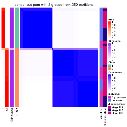
consensus_heatmap(res, k = 3)
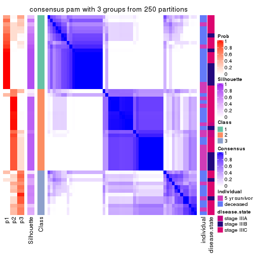
consensus_heatmap(res, k = 4)
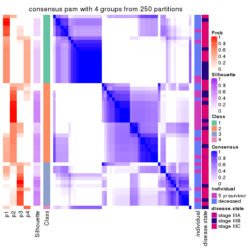
consensus_heatmap(res, k = 5)
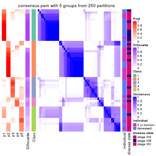
consensus_heatmap(res, k = 6)
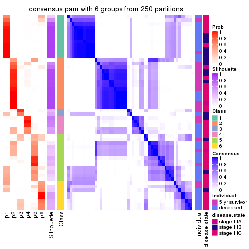
Heatmaps for the membership of samples in all partitions to see how consistent they are:
membership_heatmap(res, k = 2)
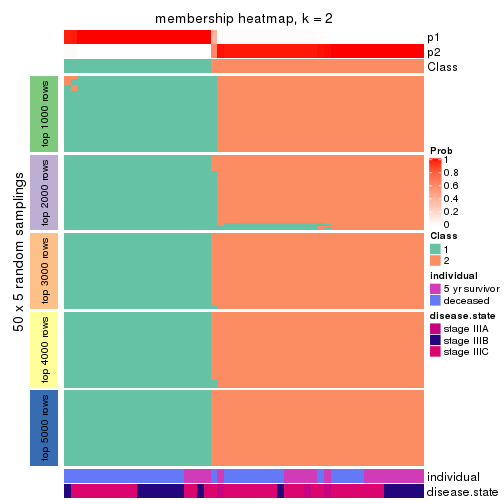
membership_heatmap(res, k = 3)
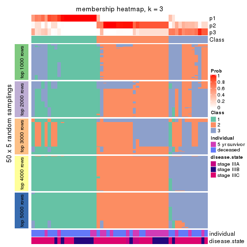
membership_heatmap(res, k = 4)
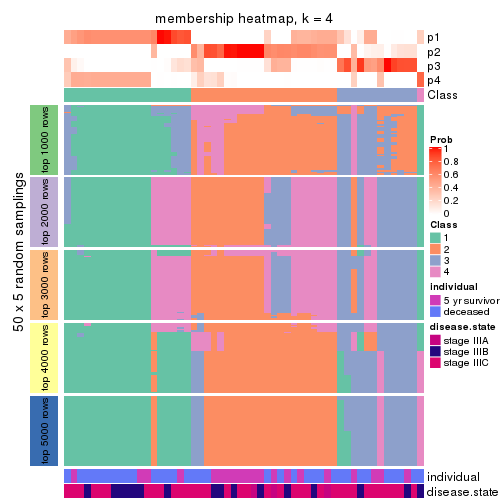
membership_heatmap(res, k = 5)
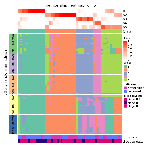
membership_heatmap(res, k = 6)
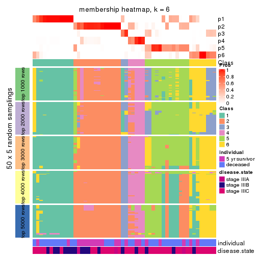
As soon as we have had the classes for columns, we can look for signatures which are significantly different between classes which can be candidate marks for certain classes. Following are the heatmaps for signatures.
Signature heatmaps where rows are scaled:
get_signatures(res, k = 2)
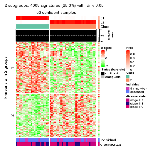
get_signatures(res, k = 3)
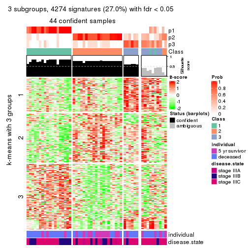
get_signatures(res, k = 4)
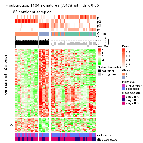
get_signatures(res, k = 5)
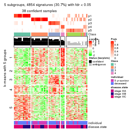
get_signatures(res, k = 6)
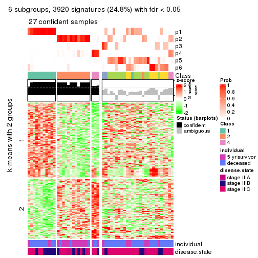
Signature heatmaps where rows are not scaled:
get_signatures(res, k = 2, scale_rows = FALSE)
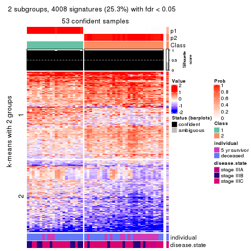
get_signatures(res, k = 3, scale_rows = FALSE)
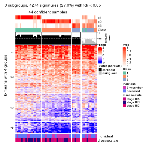
get_signatures(res, k = 4, scale_rows = FALSE)
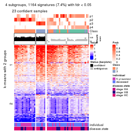
get_signatures(res, k = 5, scale_rows = FALSE)
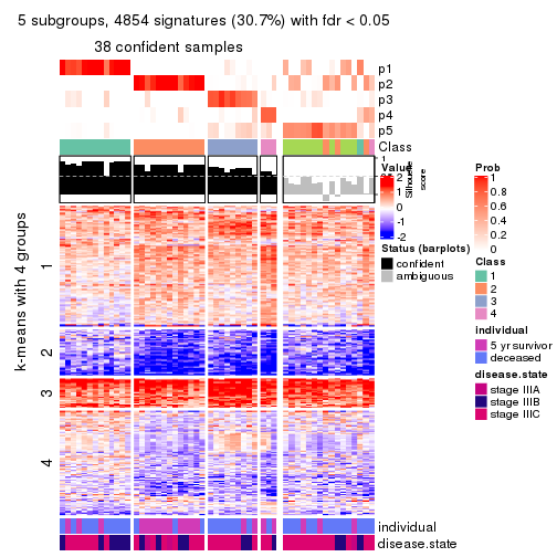
get_signatures(res, k = 6, scale_rows = FALSE)
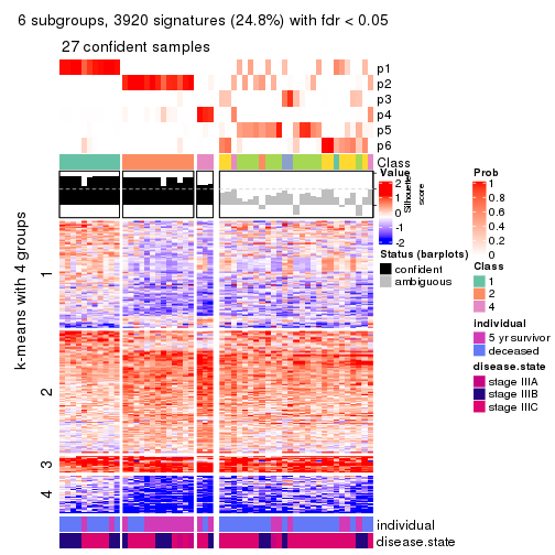
Compare the overlap of signatures from different k:
compare_signatures(res)
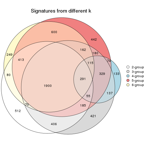
get_signature() returns a data frame invisibly. TO get the list of signatures, the function
call should be assigned to a variable explicitly. In following code, if plot argument is set
to FALSE, no heatmap is plotted while only the differential analysis is performed.
# code only for demonstration
tb = get_signature(res, k = ..., plot = FALSE)
An example of the output of tb is:
#> which_row fdr mean_1 mean_2 scaled_mean_1 scaled_mean_2 km
#> 1 38 0.042760348 8.373488 9.131774 -0.5533452 0.5164555 1
#> 2 40 0.018707592 7.106213 8.469186 -0.6173731 0.5762149 1
#> 3 55 0.019134737 10.221463 11.207825 -0.6159697 0.5749050 1
#> 4 59 0.006059896 5.921854 7.869574 -0.6899429 0.6439467 1
#> 5 60 0.018055526 8.928898 10.211722 -0.6204761 0.5791110 1
#> 6 98 0.009384629 15.714769 14.887706 0.6635654 -0.6193277 2
...
The columns in tb are:
which_row: row indices corresponding to the input matrix.fdr: FDR for the differential test. mean_x: The mean value in group x.scaled_mean_x: The mean value in group x after rows are scaled.km: Row groups if k-means clustering is applied to rows.UMAP plot which shows how samples are separated.
dimension_reduction(res, k = 2, method = "UMAP")
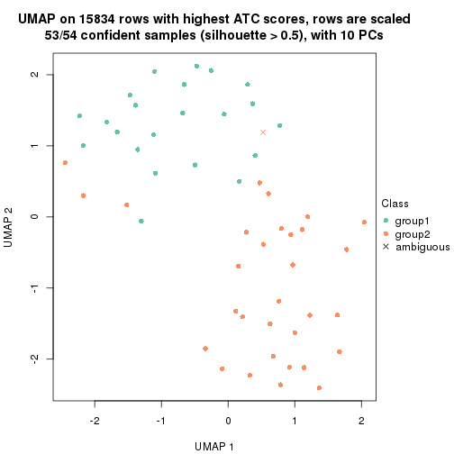
dimension_reduction(res, k = 3, method = "UMAP")
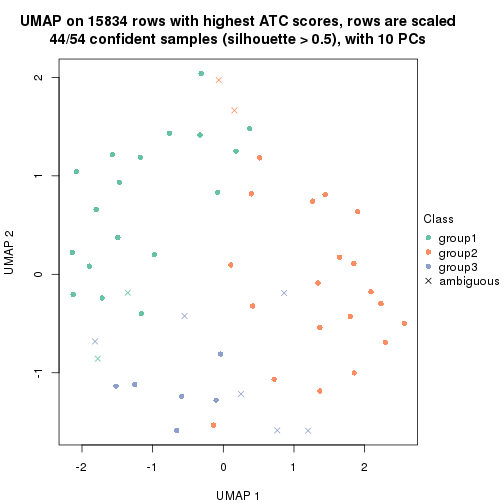
dimension_reduction(res, k = 4, method = "UMAP")
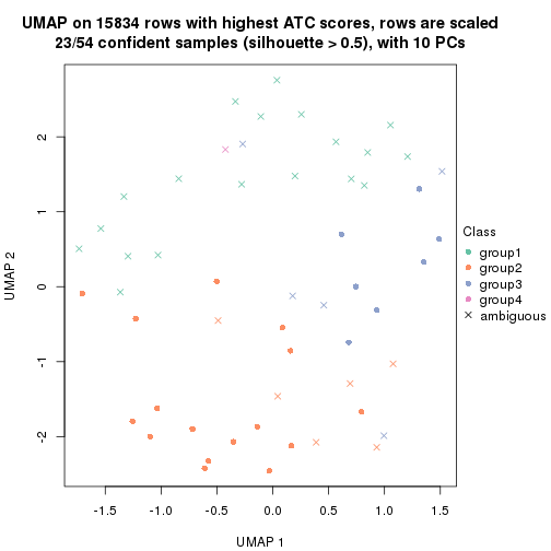
dimension_reduction(res, k = 5, method = "UMAP")
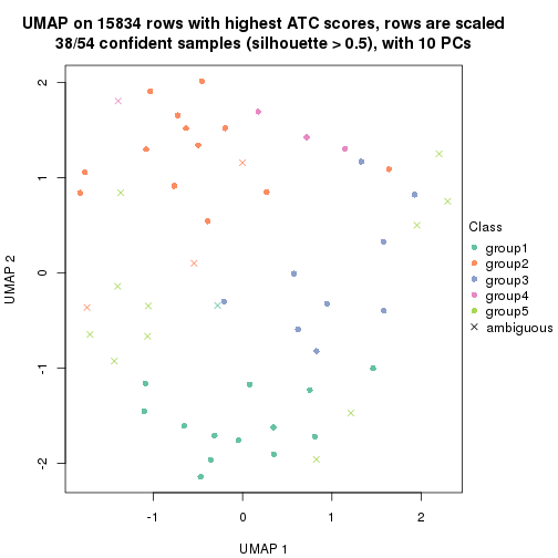
dimension_reduction(res, k = 6, method = "UMAP")
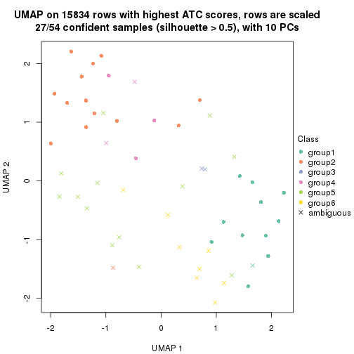
Following heatmap shows how subgroups are split when increasing k:
collect_classes(res)
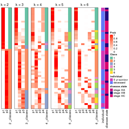
Test correlation between subgroups and known annotations. If the known annotation is numeric, one-way ANOVA test is applied, and if the known annotation is discrete, chi-squared contingency table test is applied.
test_to_known_factors(res)
#> n individual(p) disease.state(p) k
#> ATC:pam 53 0.0288 0.156 2
#> ATC:pam 44 0.0120 0.241 3
#> ATC:pam 23 0.1583 0.619 4
#> ATC:pam 38 0.0159 0.486 5
#> ATC:pam 27 0.0140 0.517 6
If matrix rows can be associated to genes, consider to use functional_enrichment(res,
...) to perform function enrichment for the signature genes. See this vignette for more detailed explanations.
The object with results only for a single top-value method and a single partition method can be extracted as:
res = res_list["ATC", "mclust"]
# you can also extract it by
# res = res_list["ATC:mclust"]
A summary of res and all the functions that can be applied to it:
res
#> A 'ConsensusPartition' object with k = 2, 3, 4, 5, 6.
#> On a matrix with 15834 rows and 54 columns.
#> Top rows (1000, 2000, 3000, 4000, 5000) are extracted by 'ATC' method.
#> Subgroups are detected by 'mclust' method.
#> Performed in total 1250 partitions by row resampling.
#> Best k for subgroups seems to be 2.
#>
#> Following methods can be applied to this 'ConsensusPartition' object:
#> [1] "cola_report" "collect_classes" "collect_plots"
#> [4] "collect_stats" "colnames" "compare_signatures"
#> [7] "consensus_heatmap" "dimension_reduction" "functional_enrichment"
#> [10] "get_anno_col" "get_anno" "get_classes"
#> [13] "get_consensus" "get_matrix" "get_membership"
#> [16] "get_param" "get_signatures" "get_stats"
#> [19] "is_best_k" "is_stable_k" "membership_heatmap"
#> [22] "ncol" "nrow" "plot_ecdf"
#> [25] "rownames" "select_partition_number" "show"
#> [28] "suggest_best_k" "test_to_known_factors"
collect_plots() function collects all the plots made from res for all k (number of partitions)
into one single page to provide an easy and fast comparison between different k.
collect_plots(res)
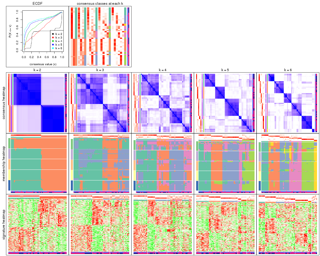
The plots are:
k and the heatmap of
predicted classes for each k.k.k.k.All the plots in panels can be made by individual functions and they are plotted later in this section.
select_partition_number() produces several plots showing different
statistics for choosing “optimized” k. There are following statistics:
k;k, the area increased is defined as \(A_k - A_{k-1}\).The detailed explanations of these statistics can be found in the cola vignette.
Generally speaking, lower PAC score, higher mean silhouette score or higher
concordance corresponds to better partition. Rand index and Jaccard index
measure how similar the current partition is compared to partition with k-1.
If they are too similar, we won't accept k is better than k-1.
select_partition_number(res)
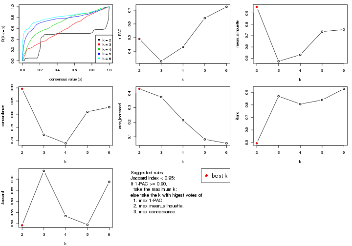
The numeric values for all these statistics can be obtained by get_stats().
get_stats(res)
#> k 1-PAC mean_silhouette concordance area_increased Rand Jaccard
#> 2 2 0.490 0.955 0.896 0.4290 0.493 0.493
#> 3 3 0.327 0.474 0.722 0.3726 0.869 0.737
#> 4 4 0.432 0.531 0.690 0.2137 0.806 0.534
#> 5 5 0.642 0.736 0.809 0.0822 0.839 0.496
#> 6 6 0.725 0.754 0.827 0.0554 0.928 0.688
suggest_best_k() suggests the best \(k\) based on these statistics. The rules are as follows:
suggest_best_k(res)
#> [1] 2
Following shows the table of the partitions (You need to click the show/hide
code output link to see it). The membership matrix (columns with name p*)
is inferred by
clue::cl_consensus()
function with the SE method. Basically the value in the membership matrix
represents the probability to belong to a certain group. The finall class
label for an item is determined with the group with highest probability it
belongs to.
In get_classes() function, the entropy is calculated from the membership
matrix and the silhouette score is calculated from the consensus matrix.
cbind(get_classes(res, k = 2), get_membership(res, k = 2))
#> class entropy silhouette p1 p2
#> GSM311939 2 0.6712 0.986 0.176 0.824
#> GSM311963 2 0.6712 0.986 0.176 0.824
#> GSM311973 1 0.2043 0.961 0.968 0.032
#> GSM311940 2 0.6801 0.986 0.180 0.820
#> GSM311953 2 0.6712 0.986 0.176 0.824
#> GSM311974 2 0.6712 0.986 0.176 0.824
#> GSM311975 2 0.6801 0.986 0.180 0.820
#> GSM311977 2 0.6801 0.986 0.180 0.820
#> GSM311982 1 0.7139 0.798 0.804 0.196
#> GSM311990 2 0.6712 0.986 0.176 0.824
#> GSM311943 1 0.0938 0.954 0.988 0.012
#> GSM311944 1 0.0000 0.952 1.000 0.000
#> GSM311946 2 0.6712 0.986 0.176 0.824
#> GSM311956 2 0.6801 0.986 0.180 0.820
#> GSM311967 2 0.6801 0.986 0.180 0.820
#> GSM311968 2 0.9427 0.702 0.360 0.640
#> GSM311972 1 0.1843 0.961 0.972 0.028
#> GSM311980 1 0.2423 0.956 0.960 0.040
#> GSM311981 1 0.3274 0.932 0.940 0.060
#> GSM311988 2 0.6712 0.986 0.176 0.824
#> GSM311957 1 0.2043 0.961 0.968 0.032
#> GSM311960 2 0.7528 0.941 0.216 0.784
#> GSM311971 1 0.2043 0.961 0.968 0.032
#> GSM311976 1 0.2043 0.961 0.968 0.032
#> GSM311978 1 0.1843 0.957 0.972 0.028
#> GSM311979 1 0.7139 0.798 0.804 0.196
#> GSM311983 1 0.7056 0.799 0.808 0.192
#> GSM311986 1 0.3879 0.917 0.924 0.076
#> GSM311991 1 0.1843 0.961 0.972 0.028
#> GSM311938 2 0.6801 0.986 0.180 0.820
#> GSM311941 2 0.6801 0.986 0.180 0.820
#> GSM311942 2 0.6712 0.986 0.176 0.824
#> GSM311945 1 0.2043 0.961 0.968 0.032
#> GSM311947 2 0.6801 0.986 0.180 0.820
#> GSM311948 2 0.6712 0.986 0.176 0.824
#> GSM311949 1 0.2043 0.961 0.968 0.032
#> GSM311950 2 0.6712 0.986 0.176 0.824
#> GSM311951 2 0.6712 0.986 0.176 0.824
#> GSM311952 1 0.0672 0.956 0.992 0.008
#> GSM311954 2 0.6801 0.986 0.180 0.820
#> GSM311955 1 0.0938 0.954 0.988 0.012
#> GSM311958 1 0.0376 0.954 0.996 0.004
#> GSM311959 1 0.0938 0.954 0.988 0.012
#> GSM311961 1 0.1843 0.961 0.972 0.028
#> GSM311962 1 0.1414 0.959 0.980 0.020
#> GSM311964 1 0.1843 0.961 0.972 0.028
#> GSM311965 2 0.6801 0.986 0.180 0.820
#> GSM311966 1 0.1843 0.957 0.972 0.028
#> GSM311969 1 0.1843 0.961 0.972 0.028
#> GSM311970 1 0.2603 0.953 0.956 0.044
#> GSM311984 2 0.6801 0.986 0.180 0.820
#> GSM311985 1 0.1843 0.961 0.972 0.028
#> GSM311987 2 0.6801 0.986 0.180 0.820
#> GSM311989 1 0.1184 0.958 0.984 0.016
cbind(get_classes(res, k = 3), get_membership(res, k = 3))
#> class entropy silhouette p1 p2 p3
#> GSM311939 2 0.8844 -0.1808 0.120 0.488 0.392
#> GSM311963 2 0.8442 0.1637 0.100 0.548 0.352
#> GSM311973 1 0.9338 -0.1830 0.468 0.172 0.360
#> GSM311940 2 0.1753 0.6651 0.048 0.952 0.000
#> GSM311953 2 0.1411 0.6668 0.036 0.964 0.000
#> GSM311974 2 0.2261 0.6691 0.000 0.932 0.068
#> GSM311975 2 0.7997 0.2723 0.084 0.600 0.316
#> GSM311977 2 0.5067 0.6522 0.052 0.832 0.116
#> GSM311982 1 0.5618 0.5111 0.732 0.008 0.260
#> GSM311990 3 0.7123 0.2098 0.032 0.364 0.604
#> GSM311943 1 0.3551 0.6568 0.868 0.000 0.132
#> GSM311944 1 0.0237 0.6861 0.996 0.000 0.004
#> GSM311946 2 0.8349 0.2434 0.108 0.584 0.308
#> GSM311956 2 0.5442 0.6545 0.056 0.812 0.132
#> GSM311967 2 0.5406 0.5431 0.012 0.764 0.224
#> GSM311968 3 0.9122 0.6607 0.280 0.184 0.536
#> GSM311972 1 0.1647 0.6844 0.960 0.004 0.036
#> GSM311980 1 0.9741 -0.3141 0.412 0.228 0.360
#> GSM311981 1 0.5845 0.4457 0.688 0.004 0.308
#> GSM311988 2 0.3573 0.6514 0.004 0.876 0.120
#> GSM311957 1 0.6737 0.4339 0.688 0.040 0.272
#> GSM311960 3 0.9914 0.4301 0.280 0.328 0.392
#> GSM311971 1 0.1999 0.6840 0.952 0.036 0.012
#> GSM311976 1 0.1491 0.6896 0.968 0.016 0.016
#> GSM311978 1 0.5553 0.5073 0.724 0.004 0.272
#> GSM311979 1 0.5618 0.5111 0.732 0.008 0.260
#> GSM311983 1 0.5216 0.5100 0.740 0.000 0.260
#> GSM311986 3 0.7575 0.2622 0.456 0.040 0.504
#> GSM311991 1 0.1647 0.6844 0.960 0.004 0.036
#> GSM311938 2 0.2773 0.6617 0.048 0.928 0.024
#> GSM311941 3 0.8379 0.6723 0.268 0.128 0.604
#> GSM311942 3 0.7898 0.6899 0.300 0.084 0.616
#> GSM311945 1 0.6143 0.3841 0.684 0.012 0.304
#> GSM311947 2 0.6109 0.5406 0.048 0.760 0.192
#> GSM311948 3 0.8892 0.1021 0.120 0.436 0.444
#> GSM311949 1 0.2651 0.6841 0.928 0.012 0.060
#> GSM311950 2 0.2066 0.6539 0.000 0.940 0.060
#> GSM311951 3 0.9072 0.6624 0.300 0.168 0.532
#> GSM311952 1 0.2878 0.6737 0.904 0.000 0.096
#> GSM311954 3 0.8089 0.6926 0.308 0.092 0.600
#> GSM311955 1 0.4235 0.6188 0.824 0.000 0.176
#> GSM311958 1 0.0592 0.6883 0.988 0.000 0.012
#> GSM311959 1 0.5216 0.5142 0.740 0.000 0.260
#> GSM311961 1 0.5873 0.4227 0.684 0.004 0.312
#> GSM311962 1 0.0424 0.6875 0.992 0.008 0.000
#> GSM311964 1 0.3349 0.6758 0.888 0.004 0.108
#> GSM311965 3 0.7949 0.6907 0.308 0.084 0.608
#> GSM311966 1 0.2878 0.6314 0.904 0.000 0.096
#> GSM311969 1 0.6509 -0.0906 0.524 0.004 0.472
#> GSM311970 1 0.9621 -0.3109 0.432 0.208 0.360
#> GSM311984 2 0.8597 0.0669 0.104 0.516 0.380
#> GSM311985 1 0.2301 0.6891 0.936 0.004 0.060
#> GSM311987 3 0.7748 0.1929 0.064 0.340 0.596
#> GSM311989 1 0.4645 0.6100 0.816 0.008 0.176
cbind(get_classes(res, k = 4), get_membership(res, k = 4))
#> class entropy silhouette p1 p2 p3 p4
#> GSM311939 3 0.1722 0.7584 0.000 0.048 0.944 0.008
#> GSM311963 4 0.6887 0.3464 0.000 0.440 0.104 0.456
#> GSM311973 4 0.8564 0.4772 0.064 0.332 0.152 0.452
#> GSM311940 2 0.1822 0.6096 0.008 0.944 0.044 0.004
#> GSM311953 2 0.1917 0.6031 0.008 0.944 0.036 0.012
#> GSM311974 2 0.4197 0.5751 0.000 0.808 0.156 0.036
#> GSM311975 2 0.7692 0.3496 0.004 0.464 0.200 0.332
#> GSM311977 2 0.3876 0.5855 0.008 0.856 0.068 0.068
#> GSM311982 1 0.4253 0.6675 0.820 0.004 0.044 0.132
#> GSM311990 3 0.1022 0.7695 0.000 0.032 0.968 0.000
#> GSM311943 1 0.2839 0.6652 0.884 0.004 0.108 0.004
#> GSM311944 1 0.0469 0.6994 0.988 0.000 0.012 0.000
#> GSM311946 2 0.7573 -0.3563 0.052 0.468 0.064 0.416
#> GSM311956 2 0.5354 0.3121 0.000 0.712 0.056 0.232
#> GSM311967 2 0.6971 0.3977 0.000 0.568 0.156 0.276
#> GSM311968 3 0.2032 0.7635 0.036 0.028 0.936 0.000
#> GSM311972 1 0.4089 0.6667 0.844 0.020 0.032 0.104
#> GSM311980 4 0.8188 0.4804 0.060 0.376 0.108 0.456
#> GSM311981 4 0.5980 0.2160 0.228 0.020 0.056 0.696
#> GSM311988 2 0.4423 0.5651 0.000 0.788 0.176 0.036
#> GSM311957 1 0.6557 0.2611 0.472 0.028 0.472 0.028
#> GSM311960 4 0.8335 0.4134 0.024 0.324 0.228 0.424
#> GSM311971 1 0.6002 0.4187 0.552 0.028 0.412 0.008
#> GSM311976 1 0.7489 0.4288 0.556 0.080 0.316 0.048
#> GSM311978 1 0.4446 0.6585 0.816 0.024 0.024 0.136
#> GSM311979 1 0.3986 0.6704 0.832 0.004 0.032 0.132
#> GSM311983 1 0.2714 0.6727 0.884 0.004 0.000 0.112
#> GSM311986 3 0.2623 0.7451 0.064 0.028 0.908 0.000
#> GSM311991 1 0.6405 0.4101 0.536 0.020 0.032 0.412
#> GSM311938 2 0.3089 0.6044 0.044 0.896 0.052 0.008
#> GSM311941 3 0.2483 0.7964 0.052 0.032 0.916 0.000
#> GSM311942 3 0.1792 0.8000 0.068 0.000 0.932 0.000
#> GSM311945 3 0.7236 0.3678 0.180 0.012 0.592 0.216
#> GSM311947 2 0.6396 0.3173 0.064 0.600 0.328 0.008
#> GSM311948 3 0.2586 0.7875 0.048 0.040 0.912 0.000
#> GSM311949 1 0.6524 0.4651 0.604 0.068 0.316 0.012
#> GSM311950 2 0.3450 0.5879 0.000 0.836 0.156 0.008
#> GSM311951 3 0.1716 0.7997 0.064 0.000 0.936 0.000
#> GSM311952 1 0.4607 0.5331 0.716 0.004 0.276 0.004
#> GSM311954 3 0.3477 0.7764 0.088 0.032 0.872 0.008
#> GSM311955 1 0.3933 0.5581 0.796 0.004 0.196 0.004
#> GSM311958 1 0.0844 0.6982 0.980 0.004 0.012 0.004
#> GSM311959 1 0.5791 -0.0322 0.556 0.024 0.416 0.004
#> GSM311961 4 0.8394 0.2825 0.132 0.064 0.332 0.472
#> GSM311962 1 0.2053 0.6905 0.924 0.000 0.072 0.004
#> GSM311964 4 0.8789 0.2714 0.176 0.072 0.308 0.444
#> GSM311965 3 0.3279 0.7762 0.096 0.032 0.872 0.000
#> GSM311966 1 0.1139 0.6997 0.972 0.008 0.012 0.008
#> GSM311969 3 0.6799 0.2547 0.392 0.020 0.532 0.056
#> GSM311970 4 0.7785 0.4564 0.080 0.412 0.052 0.456
#> GSM311984 3 0.4247 0.7485 0.044 0.040 0.848 0.068
#> GSM311985 1 0.3337 0.6781 0.888 0.020 0.032 0.060
#> GSM311987 3 0.5619 0.4613 0.320 0.040 0.640 0.000
#> GSM311989 1 0.4746 0.4540 0.632 0.000 0.368 0.000
cbind(get_classes(res, k = 5), get_membership(res, k = 5))
#> class entropy silhouette p1 p2 p3 p4 p5
#> GSM311939 3 0.2522 0.8410 0.000 0.000 0.880 0.012 0.108
#> GSM311963 5 0.2753 0.5935 0.000 0.136 0.008 0.000 0.856
#> GSM311973 5 0.2597 0.6099 0.000 0.120 0.004 0.004 0.872
#> GSM311940 2 0.1442 0.9055 0.000 0.952 0.032 0.004 0.012
#> GSM311953 2 0.0963 0.9024 0.000 0.964 0.000 0.000 0.036
#> GSM311974 2 0.2005 0.8992 0.004 0.924 0.016 0.000 0.056
#> GSM311975 2 0.4980 0.8030 0.000 0.764 0.068 0.100 0.068
#> GSM311977 2 0.1579 0.9087 0.000 0.944 0.032 0.000 0.024
#> GSM311982 1 0.1282 0.7744 0.952 0.000 0.044 0.004 0.000
#> GSM311990 3 0.1410 0.8499 0.000 0.000 0.940 0.000 0.060
#> GSM311943 3 0.6023 0.5344 0.224 0.000 0.616 0.148 0.012
#> GSM311944 1 0.3780 0.7912 0.820 0.000 0.020 0.132 0.028
#> GSM311946 5 0.6052 0.4465 0.008 0.348 0.104 0.000 0.540
#> GSM311956 2 0.1444 0.9007 0.000 0.948 0.012 0.000 0.040
#> GSM311967 2 0.3785 0.8396 0.004 0.832 0.008 0.092 0.064
#> GSM311968 3 0.2233 0.8458 0.000 0.000 0.892 0.004 0.104
#> GSM311972 4 0.3491 0.8214 0.124 0.012 0.000 0.836 0.028
#> GSM311980 5 0.2722 0.6082 0.000 0.120 0.004 0.008 0.868
#> GSM311981 4 0.1267 0.9049 0.000 0.012 0.004 0.960 0.024
#> GSM311988 2 0.1970 0.8986 0.004 0.924 0.012 0.000 0.060
#> GSM311957 5 0.7664 -0.0319 0.376 0.000 0.104 0.128 0.392
#> GSM311960 5 0.4876 0.5803 0.012 0.108 0.136 0.000 0.744
#> GSM311971 1 0.4059 0.6973 0.804 0.000 0.072 0.008 0.116
#> GSM311976 5 0.7074 0.4751 0.216 0.012 0.056 0.140 0.576
#> GSM311978 1 0.1483 0.7551 0.952 0.012 0.008 0.028 0.000
#> GSM311979 1 0.1205 0.7742 0.956 0.000 0.040 0.004 0.000
#> GSM311983 1 0.0671 0.7740 0.980 0.000 0.016 0.004 0.000
#> GSM311986 3 0.2407 0.8471 0.004 0.000 0.896 0.012 0.088
#> GSM311991 4 0.1106 0.9062 0.000 0.012 0.000 0.964 0.024
#> GSM311938 2 0.2149 0.8966 0.000 0.916 0.036 0.000 0.048
#> GSM311941 3 0.0566 0.8586 0.004 0.012 0.984 0.000 0.000
#> GSM311942 3 0.1547 0.8589 0.032 0.016 0.948 0.000 0.004
#> GSM311945 5 0.6745 0.4603 0.036 0.012 0.220 0.136 0.596
#> GSM311947 2 0.3781 0.8553 0.000 0.840 0.040 0.044 0.076
#> GSM311948 3 0.2980 0.8493 0.024 0.008 0.884 0.012 0.072
#> GSM311949 5 0.7057 0.4428 0.252 0.004 0.056 0.140 0.548
#> GSM311950 2 0.2130 0.8975 0.000 0.908 0.012 0.000 0.080
#> GSM311951 3 0.2417 0.8596 0.032 0.016 0.912 0.000 0.040
#> GSM311952 1 0.5767 0.7292 0.660 0.000 0.180 0.144 0.016
#> GSM311954 3 0.1774 0.8367 0.000 0.016 0.932 0.000 0.052
#> GSM311955 3 0.5388 0.6576 0.144 0.000 0.696 0.148 0.012
#> GSM311958 1 0.4336 0.7880 0.792 0.000 0.048 0.132 0.028
#> GSM311959 3 0.5224 0.6857 0.128 0.000 0.712 0.148 0.012
#> GSM311961 5 0.5636 0.4041 0.000 0.012 0.060 0.352 0.576
#> GSM311962 1 0.4336 0.7957 0.792 0.000 0.048 0.132 0.028
#> GSM311964 5 0.5626 0.4726 0.004 0.012 0.068 0.284 0.632
#> GSM311965 3 0.0798 0.8570 0.000 0.016 0.976 0.000 0.008
#> GSM311966 1 0.4044 0.7983 0.820 0.008 0.032 0.116 0.024
#> GSM311969 3 0.5110 0.7648 0.120 0.012 0.756 0.088 0.024
#> GSM311970 5 0.3044 0.5988 0.000 0.148 0.004 0.008 0.840
#> GSM311984 3 0.2578 0.8488 0.000 0.016 0.904 0.040 0.040
#> GSM311985 1 0.5009 0.5337 0.636 0.012 0.000 0.324 0.028
#> GSM311987 3 0.2689 0.8264 0.084 0.016 0.888 0.000 0.012
#> GSM311989 1 0.6150 0.6879 0.644 0.004 0.192 0.132 0.028
cbind(get_classes(res, k = 6), get_membership(res, k = 6))
#> class entropy silhouette p1 p2 p3 p4 p5 p6
#> GSM311939 5 0.1078 0.904 0.000 0.012 0.016 0.008 0.964 0.000
#> GSM311963 4 0.2146 0.643 0.004 0.116 0.000 0.880 0.000 0.000
#> GSM311973 4 0.1003 0.666 0.000 0.020 0.000 0.964 0.016 0.000
#> GSM311940 2 0.3229 0.804 0.004 0.856 0.048 0.016 0.004 0.072
#> GSM311953 2 0.0777 0.832 0.004 0.972 0.000 0.024 0.000 0.000
#> GSM311974 2 0.3043 0.725 0.000 0.792 0.000 0.008 0.200 0.000
#> GSM311975 2 0.3936 0.741 0.000 0.780 0.008 0.000 0.088 0.124
#> GSM311977 2 0.0260 0.832 0.000 0.992 0.000 0.008 0.000 0.000
#> GSM311982 1 0.0146 0.895 0.996 0.000 0.004 0.000 0.000 0.000
#> GSM311990 5 0.0000 0.914 0.000 0.000 0.000 0.000 1.000 0.000
#> GSM311943 3 0.3167 0.747 0.072 0.000 0.832 0.000 0.096 0.000
#> GSM311944 3 0.3512 0.682 0.248 0.000 0.740 0.004 0.008 0.000
#> GSM311946 4 0.5123 0.322 0.000 0.408 0.000 0.508 0.084 0.000
#> GSM311956 2 0.0935 0.831 0.004 0.964 0.000 0.032 0.000 0.000
#> GSM311967 2 0.3757 0.767 0.000 0.780 0.136 0.000 0.000 0.084
#> GSM311968 5 0.0551 0.911 0.000 0.004 0.004 0.008 0.984 0.000
#> GSM311972 6 0.2214 0.955 0.016 0.000 0.096 0.000 0.000 0.888
#> GSM311980 4 0.0363 0.665 0.000 0.012 0.000 0.988 0.000 0.000
#> GSM311981 6 0.1701 0.970 0.000 0.000 0.072 0.008 0.000 0.920
#> GSM311988 2 0.3984 0.433 0.000 0.596 0.000 0.008 0.396 0.000
#> GSM311957 4 0.6522 0.495 0.092 0.000 0.280 0.512 0.116 0.000
#> GSM311960 4 0.3394 0.619 0.000 0.024 0.000 0.776 0.200 0.000
#> GSM311971 1 0.1313 0.861 0.952 0.000 0.004 0.016 0.028 0.000
#> GSM311976 4 0.4820 0.618 0.088 0.000 0.256 0.652 0.004 0.000
#> GSM311978 1 0.0146 0.895 0.996 0.000 0.004 0.000 0.000 0.000
#> GSM311979 1 0.0146 0.895 0.996 0.000 0.004 0.000 0.000 0.000
#> GSM311983 1 0.0146 0.895 0.996 0.000 0.004 0.000 0.000 0.000
#> GSM311986 5 0.1226 0.888 0.000 0.004 0.040 0.004 0.952 0.000
#> GSM311991 6 0.1901 0.973 0.004 0.000 0.076 0.008 0.000 0.912
#> GSM311938 2 0.0893 0.834 0.000 0.972 0.004 0.004 0.004 0.016
#> GSM311941 5 0.1858 0.930 0.000 0.000 0.092 0.000 0.904 0.004
#> GSM311942 5 0.1806 0.931 0.000 0.000 0.088 0.000 0.908 0.004
#> GSM311945 4 0.5446 0.563 0.040 0.004 0.324 0.584 0.048 0.000
#> GSM311947 2 0.3746 0.767 0.000 0.780 0.140 0.000 0.000 0.080
#> GSM311948 5 0.0862 0.909 0.000 0.004 0.016 0.008 0.972 0.000
#> GSM311949 4 0.5125 0.581 0.108 0.000 0.276 0.612 0.004 0.000
#> GSM311950 2 0.1970 0.802 0.000 0.900 0.000 0.008 0.092 0.000
#> GSM311951 5 0.1753 0.931 0.000 0.000 0.084 0.004 0.912 0.000
#> GSM311952 3 0.3319 0.739 0.164 0.000 0.800 0.000 0.036 0.000
#> GSM311954 5 0.2003 0.923 0.000 0.000 0.116 0.000 0.884 0.000
#> GSM311955 3 0.2815 0.726 0.032 0.000 0.848 0.000 0.120 0.000
#> GSM311958 3 0.3189 0.697 0.236 0.000 0.760 0.004 0.000 0.000
#> GSM311959 3 0.2706 0.720 0.024 0.000 0.852 0.000 0.124 0.000
#> GSM311961 4 0.5214 0.518 0.004 0.000 0.112 0.596 0.000 0.288
#> GSM311962 1 0.3753 0.441 0.696 0.000 0.292 0.004 0.008 0.000
#> GSM311964 4 0.5111 0.564 0.008 0.000 0.112 0.636 0.000 0.244
#> GSM311965 5 0.2003 0.923 0.000 0.000 0.116 0.000 0.884 0.000
#> GSM311966 1 0.1958 0.804 0.896 0.000 0.100 0.004 0.000 0.000
#> GSM311969 3 0.4424 0.350 0.024 0.000 0.628 0.004 0.340 0.004
#> GSM311970 4 0.0405 0.661 0.004 0.008 0.000 0.988 0.000 0.000
#> GSM311984 5 0.2473 0.923 0.000 0.000 0.104 0.012 0.876 0.008
#> GSM311985 3 0.4348 0.641 0.124 0.000 0.724 0.000 0.000 0.152
#> GSM311987 5 0.2445 0.916 0.008 0.000 0.120 0.000 0.868 0.004
#> GSM311989 3 0.6067 0.536 0.216 0.000 0.580 0.152 0.052 0.000
Heatmaps for the consensus matrix. It visualizes the probability of two samples to be in a same group.
consensus_heatmap(res, k = 2)
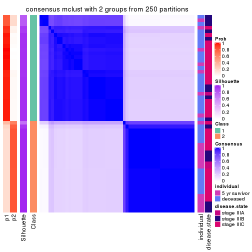
consensus_heatmap(res, k = 3)
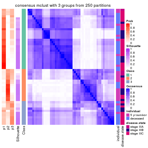
consensus_heatmap(res, k = 4)
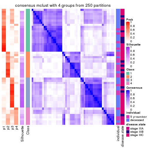
consensus_heatmap(res, k = 5)
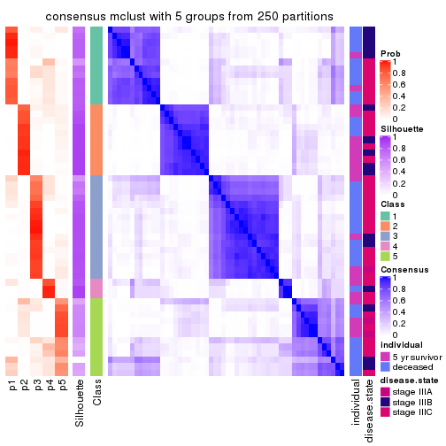
consensus_heatmap(res, k = 6)
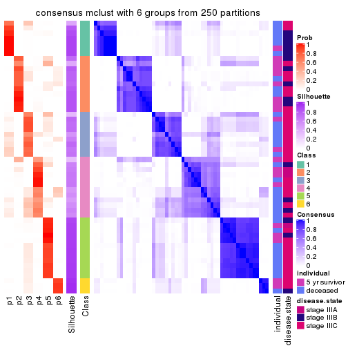
Heatmaps for the membership of samples in all partitions to see how consistent they are:
membership_heatmap(res, k = 2)
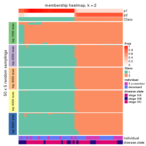
membership_heatmap(res, k = 3)
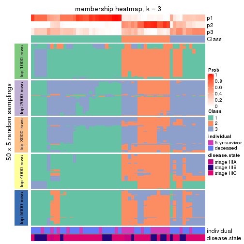
membership_heatmap(res, k = 4)
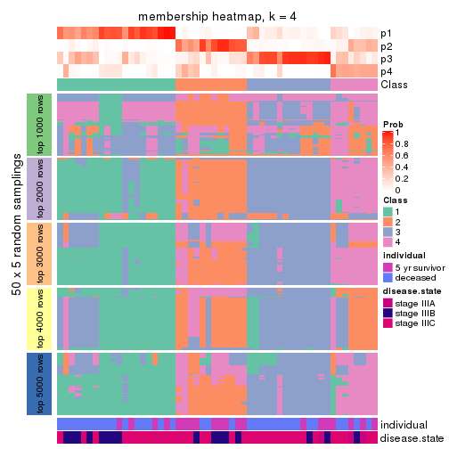
membership_heatmap(res, k = 5)
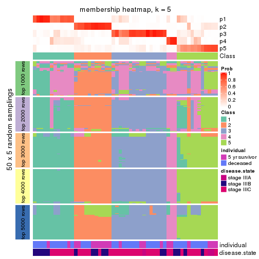
membership_heatmap(res, k = 6)
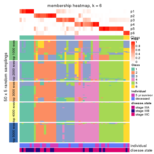
As soon as we have had the classes for columns, we can look for signatures which are significantly different between classes which can be candidate marks for certain classes. Following are the heatmaps for signatures.
Signature heatmaps where rows are scaled:
get_signatures(res, k = 2)
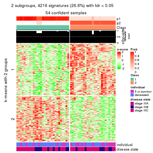
get_signatures(res, k = 3)
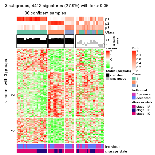
get_signatures(res, k = 4)
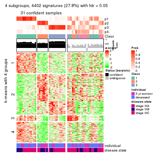
get_signatures(res, k = 5)
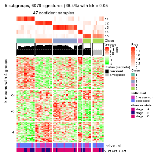
get_signatures(res, k = 6)
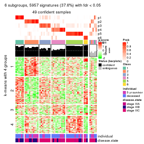
Signature heatmaps where rows are not scaled:
get_signatures(res, k = 2, scale_rows = FALSE)
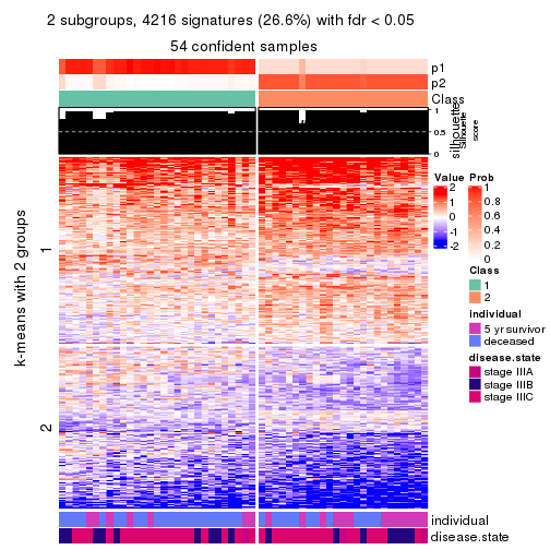
get_signatures(res, k = 3, scale_rows = FALSE)
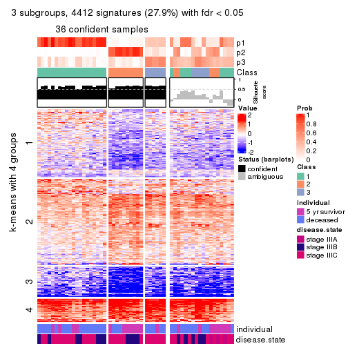
get_signatures(res, k = 4, scale_rows = FALSE)
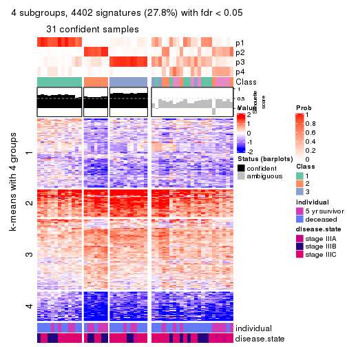
get_signatures(res, k = 5, scale_rows = FALSE)
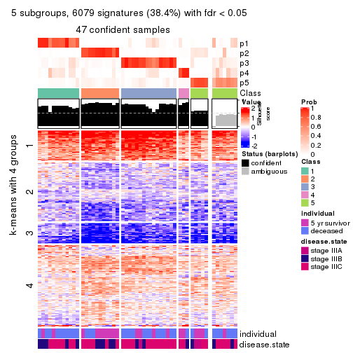
get_signatures(res, k = 6, scale_rows = FALSE)
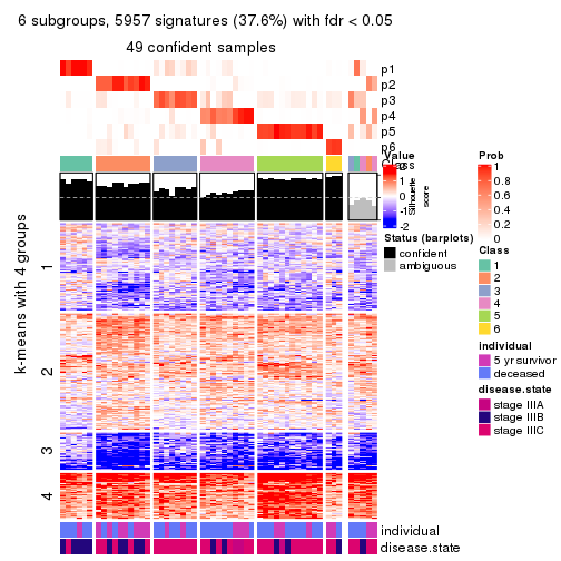
Compare the overlap of signatures from different k:
compare_signatures(res)
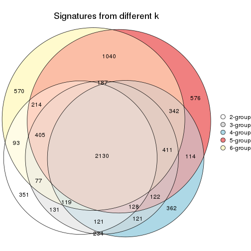
get_signature() returns a data frame invisibly. TO get the list of signatures, the function
call should be assigned to a variable explicitly. In following code, if plot argument is set
to FALSE, no heatmap is plotted while only the differential analysis is performed.
# code only for demonstration
tb = get_signature(res, k = ..., plot = FALSE)
An example of the output of tb is:
#> which_row fdr mean_1 mean_2 scaled_mean_1 scaled_mean_2 km
#> 1 38 0.042760348 8.373488 9.131774 -0.5533452 0.5164555 1
#> 2 40 0.018707592 7.106213 8.469186 -0.6173731 0.5762149 1
#> 3 55 0.019134737 10.221463 11.207825 -0.6159697 0.5749050 1
#> 4 59 0.006059896 5.921854 7.869574 -0.6899429 0.6439467 1
#> 5 60 0.018055526 8.928898 10.211722 -0.6204761 0.5791110 1
#> 6 98 0.009384629 15.714769 14.887706 0.6635654 -0.6193277 2
...
The columns in tb are:
which_row: row indices corresponding to the input matrix.fdr: FDR for the differential test. mean_x: The mean value in group x.scaled_mean_x: The mean value in group x after rows are scaled.km: Row groups if k-means clustering is applied to rows.UMAP plot which shows how samples are separated.
dimension_reduction(res, k = 2, method = "UMAP")
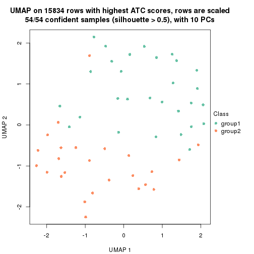
dimension_reduction(res, k = 3, method = "UMAP")
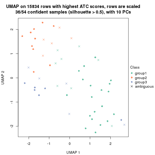
dimension_reduction(res, k = 4, method = "UMAP")
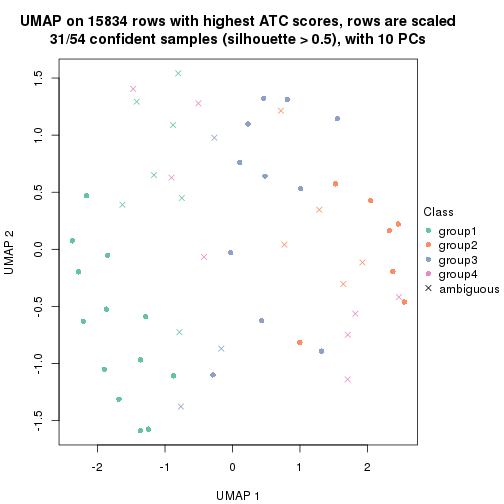
dimension_reduction(res, k = 5, method = "UMAP")
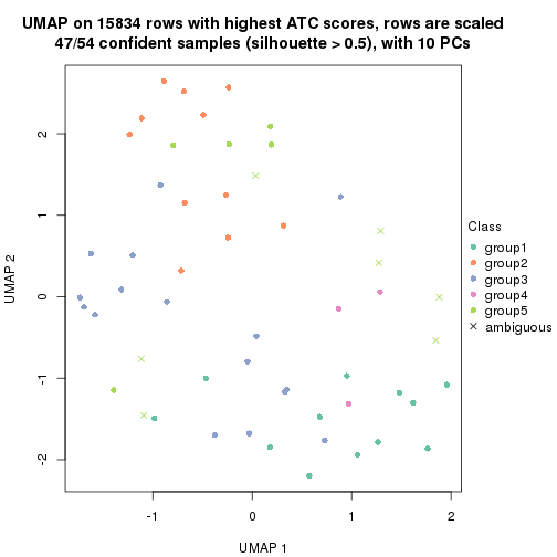
dimension_reduction(res, k = 6, method = "UMAP")
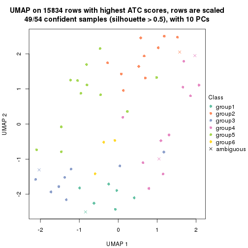
Following heatmap shows how subgroups are split when increasing k:
collect_classes(res)
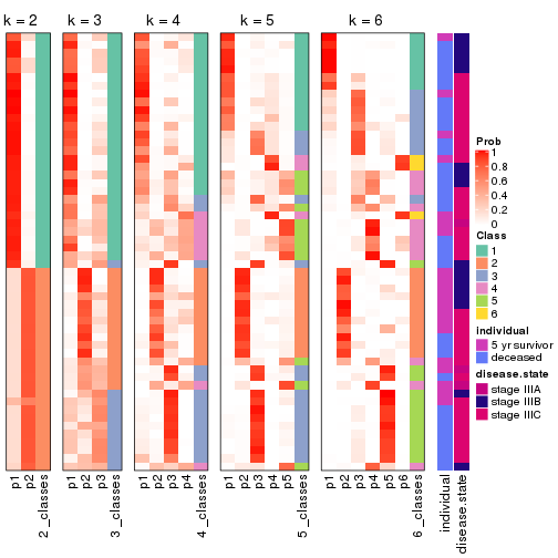
Test correlation between subgroups and known annotations. If the known annotation is numeric, one-way ANOVA test is applied, and if the known annotation is discrete, chi-squared contingency table test is applied.
test_to_known_factors(res)
#> n individual(p) disease.state(p) k
#> ATC:mclust 54 0.0670 0.7606 2
#> ATC:mclust 36 0.0150 0.1973 3
#> ATC:mclust 31 0.1281 0.3407 4
#> ATC:mclust 47 0.0288 0.0557 5
#> ATC:mclust 49 0.1386 0.0345 6
If matrix rows can be associated to genes, consider to use functional_enrichment(res,
...) to perform function enrichment for the signature genes. See this vignette for more detailed explanations.
The object with results only for a single top-value method and a single partition method can be extracted as:
res = res_list["ATC", "NMF"]
# you can also extract it by
# res = res_list["ATC:NMF"]
A summary of res and all the functions that can be applied to it:
res
#> A 'ConsensusPartition' object with k = 2, 3, 4, 5, 6.
#> On a matrix with 15834 rows and 54 columns.
#> Top rows (1000, 2000, 3000, 4000, 5000) are extracted by 'ATC' method.
#> Subgroups are detected by 'NMF' method.
#> Performed in total 1250 partitions by row resampling.
#> Best k for subgroups seems to be 2.
#>
#> Following methods can be applied to this 'ConsensusPartition' object:
#> [1] "cola_report" "collect_classes" "collect_plots"
#> [4] "collect_stats" "colnames" "compare_signatures"
#> [7] "consensus_heatmap" "dimension_reduction" "functional_enrichment"
#> [10] "get_anno_col" "get_anno" "get_classes"
#> [13] "get_consensus" "get_matrix" "get_membership"
#> [16] "get_param" "get_signatures" "get_stats"
#> [19] "is_best_k" "is_stable_k" "membership_heatmap"
#> [22] "ncol" "nrow" "plot_ecdf"
#> [25] "rownames" "select_partition_number" "show"
#> [28] "suggest_best_k" "test_to_known_factors"
collect_plots() function collects all the plots made from res for all k (number of partitions)
into one single page to provide an easy and fast comparison between different k.
collect_plots(res)
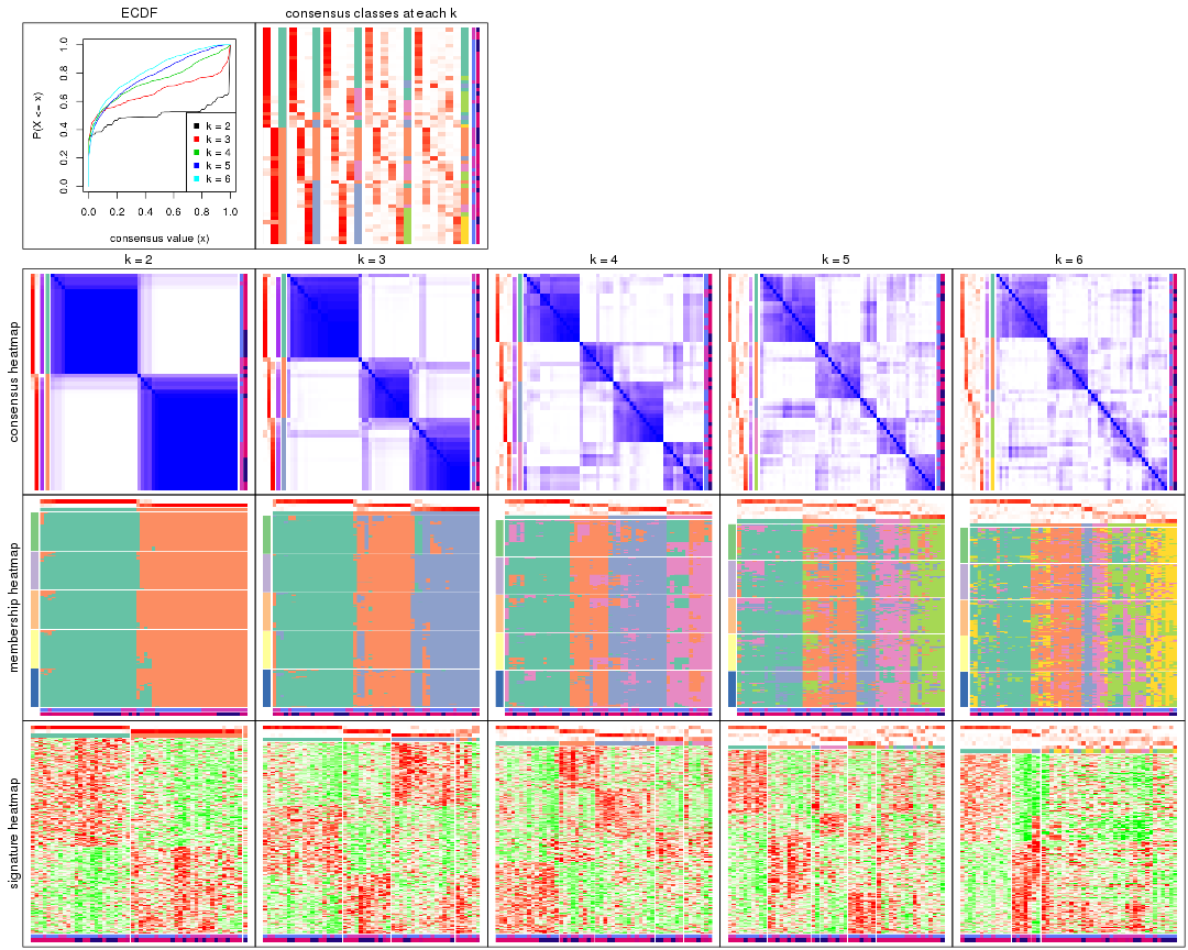
The plots are:
k and the heatmap of
predicted classes for each k.k.k.k.All the plots in panels can be made by individual functions and they are plotted later in this section.
select_partition_number() produces several plots showing different
statistics for choosing “optimized” k. There are following statistics:
k;k, the area increased is defined as \(A_k - A_{k-1}\).The detailed explanations of these statistics can be found in the cola vignette.
Generally speaking, lower PAC score, higher mean silhouette score or higher
concordance corresponds to better partition. Rand index and Jaccard index
measure how similar the current partition is compared to partition with k-1.
If they are too similar, we won't accept k is better than k-1.
select_partition_number(res)
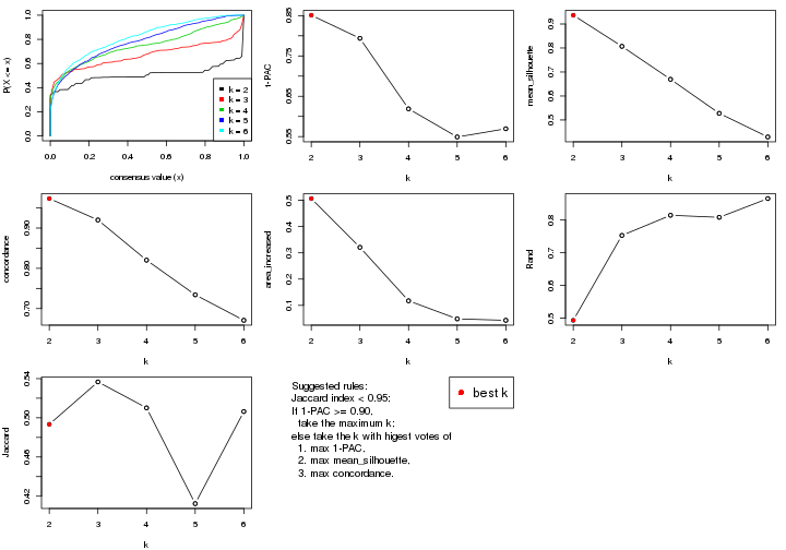
The numeric values for all these statistics can be obtained by get_stats().
get_stats(res)
#> k 1-PAC mean_silhouette concordance area_increased Rand Jaccard
#> 2 2 0.851 0.937 0.973 0.5065 0.493 0.493
#> 3 3 0.794 0.807 0.920 0.3209 0.753 0.537
#> 4 4 0.619 0.670 0.820 0.1175 0.814 0.510
#> 5 5 0.549 0.528 0.734 0.0486 0.808 0.412
#> 6 6 0.569 0.429 0.671 0.0432 0.865 0.506
suggest_best_k() suggests the best \(k\) based on these statistics. The rules are as follows:
suggest_best_k(res)
#> [1] 2
Following shows the table of the partitions (You need to click the show/hide
code output link to see it). The membership matrix (columns with name p*)
is inferred by
clue::cl_consensus()
function with the SE method. Basically the value in the membership matrix
represents the probability to belong to a certain group. The finall class
label for an item is determined with the group with highest probability it
belongs to.
In get_classes() function, the entropy is calculated from the membership
matrix and the silhouette score is calculated from the consensus matrix.
cbind(get_classes(res, k = 2), get_membership(res, k = 2))
#> class entropy silhouette p1 p2
#> GSM311939 2 0.0000 0.9622 0.000 1.000
#> GSM311963 2 0.0000 0.9622 0.000 1.000
#> GSM311973 1 0.4815 0.8866 0.896 0.104
#> GSM311940 2 0.0000 0.9622 0.000 1.000
#> GSM311953 2 0.0000 0.9622 0.000 1.000
#> GSM311974 2 0.0000 0.9622 0.000 1.000
#> GSM311975 2 0.0000 0.9622 0.000 1.000
#> GSM311977 2 0.0000 0.9622 0.000 1.000
#> GSM311982 1 0.0000 0.9817 1.000 0.000
#> GSM311990 2 0.0000 0.9622 0.000 1.000
#> GSM311943 1 0.0000 0.9817 1.000 0.000
#> GSM311944 1 0.0000 0.9817 1.000 0.000
#> GSM311946 2 0.0000 0.9622 0.000 1.000
#> GSM311956 2 0.0000 0.9622 0.000 1.000
#> GSM311967 2 0.0000 0.9622 0.000 1.000
#> GSM311968 2 0.1414 0.9466 0.020 0.980
#> GSM311972 1 0.0000 0.9817 1.000 0.000
#> GSM311980 2 0.6531 0.7966 0.168 0.832
#> GSM311981 2 0.7453 0.7355 0.212 0.788
#> GSM311988 2 0.0000 0.9622 0.000 1.000
#> GSM311957 1 0.0000 0.9817 1.000 0.000
#> GSM311960 2 0.0376 0.9594 0.004 0.996
#> GSM311971 1 0.0000 0.9817 1.000 0.000
#> GSM311976 1 0.0000 0.9817 1.000 0.000
#> GSM311978 1 0.0000 0.9817 1.000 0.000
#> GSM311979 1 0.0000 0.9817 1.000 0.000
#> GSM311983 1 0.0000 0.9817 1.000 0.000
#> GSM311986 2 0.9998 0.0259 0.492 0.508
#> GSM311991 1 0.0000 0.9817 1.000 0.000
#> GSM311938 2 0.0000 0.9622 0.000 1.000
#> GSM311941 2 0.0000 0.9622 0.000 1.000
#> GSM311942 2 0.0000 0.9622 0.000 1.000
#> GSM311945 1 0.2603 0.9460 0.956 0.044
#> GSM311947 2 0.0000 0.9622 0.000 1.000
#> GSM311948 2 0.0000 0.9622 0.000 1.000
#> GSM311949 1 0.0000 0.9817 1.000 0.000
#> GSM311950 2 0.0000 0.9622 0.000 1.000
#> GSM311951 2 0.0000 0.9622 0.000 1.000
#> GSM311952 1 0.0000 0.9817 1.000 0.000
#> GSM311954 2 0.0000 0.9622 0.000 1.000
#> GSM311955 1 0.0000 0.9817 1.000 0.000
#> GSM311958 1 0.0000 0.9817 1.000 0.000
#> GSM311959 1 0.0000 0.9817 1.000 0.000
#> GSM311961 1 0.6623 0.7965 0.828 0.172
#> GSM311962 1 0.0000 0.9817 1.000 0.000
#> GSM311964 1 0.0000 0.9817 1.000 0.000
#> GSM311965 2 0.0000 0.9622 0.000 1.000
#> GSM311966 1 0.0000 0.9817 1.000 0.000
#> GSM311969 1 0.4690 0.8913 0.900 0.100
#> GSM311970 2 0.5519 0.8441 0.128 0.872
#> GSM311984 2 0.0000 0.9622 0.000 1.000
#> GSM311985 1 0.0000 0.9817 1.000 0.000
#> GSM311987 2 0.0000 0.9622 0.000 1.000
#> GSM311989 1 0.0000 0.9817 1.000 0.000
cbind(get_classes(res, k = 3), get_membership(res, k = 3))
#> class entropy silhouette p1 p2 p3
#> GSM311939 3 0.0237 0.87397 0.000 0.004 0.996
#> GSM311963 2 0.0747 0.85576 0.000 0.984 0.016
#> GSM311973 1 0.6680 0.00541 0.508 0.484 0.008
#> GSM311940 2 0.1753 0.84602 0.000 0.952 0.048
#> GSM311953 2 0.1643 0.84762 0.000 0.956 0.044
#> GSM311974 3 0.4931 0.64224 0.000 0.232 0.768
#> GSM311975 2 0.0592 0.85586 0.000 0.988 0.012
#> GSM311977 2 0.0237 0.85655 0.000 0.996 0.004
#> GSM311982 1 0.0000 0.95741 1.000 0.000 0.000
#> GSM311990 3 0.0000 0.87453 0.000 0.000 1.000
#> GSM311943 1 0.1860 0.91765 0.948 0.000 0.052
#> GSM311944 1 0.0000 0.95741 1.000 0.000 0.000
#> GSM311946 2 0.1753 0.84590 0.000 0.952 0.048
#> GSM311956 2 0.0237 0.85655 0.000 0.996 0.004
#> GSM311967 3 0.6260 0.22013 0.000 0.448 0.552
#> GSM311968 3 0.0000 0.87453 0.000 0.000 1.000
#> GSM311972 1 0.1411 0.93567 0.964 0.036 0.000
#> GSM311980 2 0.0000 0.85564 0.000 1.000 0.000
#> GSM311981 2 0.0424 0.85487 0.008 0.992 0.000
#> GSM311988 3 0.5760 0.44574 0.000 0.328 0.672
#> GSM311957 1 0.0983 0.94898 0.980 0.004 0.016
#> GSM311960 2 0.5115 0.71253 0.016 0.796 0.188
#> GSM311971 1 0.0237 0.95657 0.996 0.004 0.000
#> GSM311976 1 0.0892 0.95029 0.980 0.020 0.000
#> GSM311978 1 0.0000 0.95741 1.000 0.000 0.000
#> GSM311979 1 0.0000 0.95741 1.000 0.000 0.000
#> GSM311983 1 0.0000 0.95741 1.000 0.000 0.000
#> GSM311986 3 0.0592 0.86976 0.012 0.000 0.988
#> GSM311991 1 0.2066 0.91672 0.940 0.060 0.000
#> GSM311938 2 0.5968 0.38001 0.000 0.636 0.364
#> GSM311941 3 0.0000 0.87453 0.000 0.000 1.000
#> GSM311942 3 0.0000 0.87453 0.000 0.000 1.000
#> GSM311945 1 0.0592 0.95406 0.988 0.012 0.000
#> GSM311947 3 0.1860 0.85695 0.000 0.052 0.948
#> GSM311948 3 0.1031 0.86978 0.000 0.024 0.976
#> GSM311949 1 0.0592 0.95406 0.988 0.012 0.000
#> GSM311950 3 0.0747 0.87263 0.000 0.016 0.984
#> GSM311951 3 0.0000 0.87453 0.000 0.000 1.000
#> GSM311952 1 0.0000 0.95741 1.000 0.000 0.000
#> GSM311954 3 0.2165 0.84982 0.000 0.064 0.936
#> GSM311955 1 0.2625 0.88353 0.916 0.000 0.084
#> GSM311958 1 0.0000 0.95741 1.000 0.000 0.000
#> GSM311959 3 0.4974 0.66825 0.236 0.000 0.764
#> GSM311961 2 0.3267 0.77583 0.116 0.884 0.000
#> GSM311962 1 0.0000 0.95741 1.000 0.000 0.000
#> GSM311964 2 0.6291 0.01610 0.468 0.532 0.000
#> GSM311965 3 0.3425 0.81033 0.004 0.112 0.884
#> GSM311966 1 0.0000 0.95741 1.000 0.000 0.000
#> GSM311969 3 0.5327 0.62460 0.272 0.000 0.728
#> GSM311970 2 0.0000 0.85564 0.000 1.000 0.000
#> GSM311984 2 0.6026 0.35132 0.000 0.624 0.376
#> GSM311985 1 0.0237 0.95638 0.996 0.004 0.000
#> GSM311987 3 0.0000 0.87453 0.000 0.000 1.000
#> GSM311989 1 0.0237 0.95657 0.996 0.004 0.000
cbind(get_classes(res, k = 4), get_membership(res, k = 4))
#> class entropy silhouette p1 p2 p3 p4
#> GSM311939 3 0.3547 0.8050 0.000 0.016 0.840 0.144
#> GSM311963 4 0.4356 0.2941 0.000 0.292 0.000 0.708
#> GSM311973 4 0.1661 0.6098 0.052 0.000 0.004 0.944
#> GSM311940 2 0.3486 0.7483 0.000 0.812 0.000 0.188
#> GSM311953 2 0.4673 0.6476 0.000 0.700 0.008 0.292
#> GSM311974 3 0.5308 0.6490 0.000 0.036 0.684 0.280
#> GSM311975 2 0.0336 0.7368 0.008 0.992 0.000 0.000
#> GSM311977 2 0.3837 0.7231 0.000 0.776 0.000 0.224
#> GSM311982 1 0.2216 0.7931 0.908 0.000 0.000 0.092
#> GSM311990 3 0.0000 0.8436 0.000 0.000 1.000 0.000
#> GSM311943 1 0.0524 0.8502 0.988 0.000 0.004 0.008
#> GSM311944 1 0.0376 0.8517 0.992 0.000 0.004 0.004
#> GSM311946 4 0.4989 -0.2471 0.000 0.472 0.000 0.528
#> GSM311956 2 0.3444 0.7489 0.000 0.816 0.000 0.184
#> GSM311967 2 0.2011 0.7118 0.000 0.920 0.080 0.000
#> GSM311968 3 0.3123 0.7744 0.000 0.000 0.844 0.156
#> GSM311972 1 0.4904 0.6847 0.744 0.216 0.000 0.040
#> GSM311980 4 0.2530 0.5350 0.000 0.112 0.000 0.888
#> GSM311981 2 0.2032 0.7022 0.028 0.936 0.000 0.036
#> GSM311988 3 0.5523 0.5465 0.000 0.024 0.596 0.380
#> GSM311957 4 0.4356 0.5752 0.292 0.000 0.000 0.708
#> GSM311960 4 0.1639 0.5749 0.004 0.036 0.008 0.952
#> GSM311971 4 0.4933 0.3626 0.432 0.000 0.000 0.568
#> GSM311976 4 0.4543 0.5492 0.324 0.000 0.000 0.676
#> GSM311978 1 0.0188 0.8513 0.996 0.000 0.000 0.004
#> GSM311979 1 0.2011 0.8054 0.920 0.000 0.000 0.080
#> GSM311983 1 0.0188 0.8513 0.996 0.000 0.000 0.004
#> GSM311986 3 0.0921 0.8425 0.000 0.000 0.972 0.028
#> GSM311991 1 0.4956 0.6720 0.732 0.232 0.000 0.036
#> GSM311938 2 0.3051 0.7622 0.000 0.884 0.028 0.088
#> GSM311941 3 0.0524 0.8427 0.004 0.000 0.988 0.008
#> GSM311942 3 0.0000 0.8436 0.000 0.000 1.000 0.000
#> GSM311945 4 0.3726 0.6449 0.212 0.000 0.000 0.788
#> GSM311947 3 0.3528 0.7617 0.000 0.192 0.808 0.000
#> GSM311948 3 0.2124 0.8355 0.000 0.028 0.932 0.040
#> GSM311949 4 0.4933 0.3673 0.432 0.000 0.000 0.568
#> GSM311950 3 0.1042 0.8446 0.000 0.008 0.972 0.020
#> GSM311951 3 0.4715 0.7676 0.012 0.024 0.776 0.188
#> GSM311952 1 0.0469 0.8491 0.988 0.000 0.000 0.012
#> GSM311954 3 0.5468 0.6729 0.024 0.248 0.708 0.020
#> GSM311955 1 0.1394 0.8434 0.964 0.008 0.012 0.016
#> GSM311958 1 0.0000 0.8514 1.000 0.000 0.000 0.000
#> GSM311959 1 0.5126 0.7040 0.776 0.048 0.156 0.020
#> GSM311961 2 0.4399 0.5609 0.224 0.760 0.000 0.016
#> GSM311962 1 0.1940 0.8088 0.924 0.000 0.000 0.076
#> GSM311964 4 0.6474 0.5988 0.256 0.120 0.000 0.624
#> GSM311965 3 0.5537 0.6953 0.064 0.200 0.728 0.008
#> GSM311966 1 0.0336 0.8506 0.992 0.000 0.000 0.008
#> GSM311969 1 0.6670 0.6297 0.680 0.192 0.084 0.044
#> GSM311970 4 0.4431 0.2929 0.000 0.304 0.000 0.696
#> GSM311984 2 0.7442 0.3439 0.000 0.476 0.340 0.184
#> GSM311985 1 0.1716 0.8274 0.936 0.064 0.000 0.000
#> GSM311987 3 0.0657 0.8428 0.000 0.004 0.984 0.012
#> GSM311989 1 0.4916 0.0184 0.576 0.000 0.000 0.424
cbind(get_classes(res, k = 5), get_membership(res, k = 5))
#> class entropy silhouette p1 p2 p3 p4 p5
#> GSM311939 5 0.497 0.6170 0.000 0.080 0.012 0.184 0.724
#> GSM311963 4 0.295 0.5959 0.000 0.144 0.012 0.844 0.000
#> GSM311973 4 0.390 0.6984 0.216 0.012 0.008 0.764 0.000
#> GSM311940 2 0.120 0.7137 0.000 0.960 0.012 0.028 0.000
#> GSM311953 2 0.448 0.6087 0.000 0.732 0.008 0.224 0.036
#> GSM311974 2 0.533 0.5349 0.004 0.640 0.004 0.060 0.292
#> GSM311975 2 0.249 0.6894 0.000 0.872 0.124 0.004 0.000
#> GSM311977 2 0.251 0.7005 0.000 0.892 0.028 0.080 0.000
#> GSM311982 1 0.180 0.5618 0.932 0.000 0.020 0.048 0.000
#> GSM311990 5 0.130 0.7297 0.000 0.016 0.028 0.000 0.956
#> GSM311943 1 0.419 0.5545 0.708 0.000 0.276 0.004 0.012
#> GSM311944 1 0.409 0.5815 0.736 0.000 0.244 0.004 0.016
#> GSM311946 2 0.488 0.4058 0.000 0.600 0.004 0.372 0.024
#> GSM311956 2 0.304 0.6945 0.000 0.860 0.100 0.040 0.000
#> GSM311967 2 0.449 0.6370 0.000 0.740 0.204 0.004 0.052
#> GSM311968 5 0.600 0.4768 0.264 0.008 0.032 0.064 0.632
#> GSM311972 3 0.505 0.1040 0.408 0.028 0.560 0.004 0.000
#> GSM311980 4 0.519 0.6958 0.184 0.076 0.024 0.716 0.000
#> GSM311981 3 0.373 0.3504 0.000 0.216 0.768 0.016 0.000
#> GSM311988 4 0.541 0.3487 0.000 0.080 0.012 0.664 0.244
#> GSM311957 4 0.481 0.5803 0.340 0.000 0.008 0.632 0.020
#> GSM311960 4 0.541 0.6740 0.240 0.056 0.016 0.680 0.008
#> GSM311971 1 0.301 0.4785 0.824 0.000 0.004 0.172 0.000
#> GSM311976 4 0.349 0.6672 0.212 0.000 0.008 0.780 0.000
#> GSM311978 1 0.377 0.5667 0.728 0.000 0.268 0.004 0.000
#> GSM311979 1 0.217 0.5944 0.912 0.000 0.064 0.024 0.000
#> GSM311983 1 0.389 0.5624 0.724 0.000 0.268 0.008 0.000
#> GSM311986 5 0.230 0.7216 0.000 0.000 0.048 0.044 0.908
#> GSM311991 3 0.341 0.5465 0.116 0.020 0.844 0.020 0.000
#> GSM311938 2 0.251 0.7136 0.000 0.908 0.044 0.024 0.024
#> GSM311941 5 0.479 0.6010 0.044 0.168 0.028 0.004 0.756
#> GSM311942 5 0.527 0.5755 0.224 0.028 0.028 0.016 0.704
#> GSM311945 1 0.467 0.4440 0.796 0.024 0.028 0.104 0.048
#> GSM311947 2 0.529 0.2912 0.000 0.544 0.052 0.000 0.404
#> GSM311948 2 0.601 0.5627 0.028 0.656 0.032 0.044 0.240
#> GSM311949 1 0.362 0.5529 0.816 0.000 0.048 0.136 0.000
#> GSM311950 5 0.415 0.7100 0.000 0.040 0.052 0.092 0.816
#> GSM311951 1 0.755 -0.1252 0.484 0.304 0.028 0.036 0.148
#> GSM311952 1 0.296 0.6062 0.840 0.000 0.152 0.004 0.004
#> GSM311954 5 0.628 0.2846 0.004 0.116 0.384 0.004 0.492
#> GSM311955 1 0.523 0.0255 0.488 0.008 0.480 0.004 0.020
#> GSM311958 1 0.413 0.3693 0.620 0.000 0.380 0.000 0.000
#> GSM311959 3 0.592 0.5130 0.140 0.008 0.636 0.004 0.212
#> GSM311961 2 0.640 0.1979 0.168 0.572 0.244 0.016 0.000
#> GSM311962 1 0.358 0.6039 0.792 0.000 0.192 0.012 0.004
#> GSM311964 4 0.711 0.4803 0.296 0.068 0.124 0.512 0.000
#> GSM311965 2 0.584 0.5589 0.052 0.664 0.036 0.012 0.236
#> GSM311966 1 0.384 0.5488 0.716 0.000 0.280 0.004 0.000
#> GSM311969 3 0.643 0.4097 0.296 0.040 0.568 0.000 0.096
#> GSM311970 4 0.478 0.5967 0.012 0.132 0.104 0.752 0.000
#> GSM311984 2 0.579 0.6269 0.004 0.684 0.060 0.196 0.056
#> GSM311985 1 0.427 0.4503 0.648 0.008 0.344 0.000 0.000
#> GSM311987 5 0.305 0.7099 0.000 0.060 0.076 0.000 0.864
#> GSM311989 1 0.341 0.4952 0.844 0.000 0.016 0.116 0.024
cbind(get_classes(res, k = 6), get_membership(res, k = 6))
#> class entropy silhouette p1 p2 p3 p4 p5 p6
#> GSM311939 4 0.581 -0.00698 0.000 0.092 0.000 0.460 0.028 0.420
#> GSM311963 4 0.580 0.42936 0.000 0.108 0.028 0.540 0.324 0.000
#> GSM311973 5 0.330 0.23125 0.000 0.000 0.024 0.188 0.788 0.000
#> GSM311940 2 0.137 0.62369 0.000 0.944 0.012 0.044 0.000 0.000
#> GSM311953 2 0.381 0.48941 0.000 0.736 0.000 0.228 0.036 0.000
#> GSM311974 2 0.633 0.43154 0.000 0.576 0.012 0.200 0.048 0.164
#> GSM311975 2 0.313 0.61898 0.004 0.848 0.084 0.060 0.000 0.004
#> GSM311977 2 0.277 0.61498 0.000 0.872 0.076 0.040 0.012 0.000
#> GSM311982 1 0.426 0.10086 0.560 0.000 0.012 0.004 0.424 0.000
#> GSM311990 6 0.202 0.48581 0.000 0.008 0.000 0.096 0.000 0.896
#> GSM311943 1 0.155 0.74902 0.944 0.000 0.012 0.032 0.004 0.008
#> GSM311944 1 0.225 0.73491 0.912 0.000 0.008 0.024 0.044 0.012
#> GSM311946 2 0.509 0.34556 0.000 0.628 0.004 0.252 0.116 0.000
#> GSM311956 2 0.399 0.55286 0.000 0.756 0.192 0.016 0.036 0.000
#> GSM311967 2 0.625 0.44472 0.000 0.560 0.236 0.068 0.000 0.136
#> GSM311968 5 0.667 0.14454 0.012 0.012 0.016 0.184 0.484 0.292
#> GSM311972 1 0.445 0.62290 0.720 0.020 0.216 0.040 0.000 0.004
#> GSM311980 5 0.431 0.32916 0.000 0.084 0.052 0.088 0.776 0.000
#> GSM311981 3 0.176 0.58205 0.000 0.096 0.904 0.000 0.000 0.000
#> GSM311988 4 0.656 0.44665 0.000 0.100 0.000 0.544 0.192 0.164
#> GSM311957 5 0.471 0.34627 0.052 0.000 0.012 0.188 0.724 0.024
#> GSM311960 5 0.313 0.37165 0.008 0.052 0.000 0.096 0.844 0.000
#> GSM311971 5 0.498 0.09226 0.448 0.000 0.008 0.048 0.496 0.000
#> GSM311976 5 0.557 -0.15595 0.052 0.000 0.048 0.356 0.544 0.000
#> GSM311978 1 0.162 0.74285 0.936 0.000 0.012 0.008 0.044 0.000
#> GSM311979 1 0.354 0.59699 0.764 0.000 0.020 0.004 0.212 0.000
#> GSM311983 1 0.241 0.74910 0.904 0.000 0.024 0.048 0.016 0.008
#> GSM311986 6 0.237 0.49022 0.004 0.000 0.008 0.092 0.008 0.888
#> GSM311991 3 0.225 0.60873 0.072 0.000 0.900 0.012 0.016 0.000
#> GSM311938 2 0.341 0.61095 0.000 0.820 0.016 0.128 0.000 0.036
#> GSM311941 6 0.682 0.29531 0.028 0.196 0.008 0.168 0.044 0.556
#> GSM311942 6 0.676 0.08617 0.004 0.044 0.008 0.160 0.316 0.468
#> GSM311945 5 0.576 0.35529 0.340 0.044 0.008 0.056 0.552 0.000
#> GSM311947 2 0.521 0.30610 0.000 0.548 0.012 0.068 0.000 0.372
#> GSM311948 2 0.655 0.45377 0.000 0.592 0.020 0.156 0.092 0.140
#> GSM311949 1 0.474 0.58051 0.716 0.000 0.020 0.116 0.148 0.000
#> GSM311950 6 0.551 0.32780 0.000 0.052 0.052 0.240 0.012 0.644
#> GSM311951 5 0.871 0.08664 0.128 0.292 0.012 0.152 0.312 0.104
#> GSM311952 1 0.167 0.74851 0.940 0.000 0.012 0.028 0.016 0.004
#> GSM311954 6 0.670 0.43556 0.064 0.068 0.080 0.184 0.004 0.600
#> GSM311955 1 0.512 0.60495 0.704 0.000 0.044 0.152 0.004 0.096
#> GSM311958 1 0.380 0.71268 0.804 0.000 0.132 0.028 0.028 0.008
#> GSM311959 6 0.749 0.15681 0.276 0.004 0.192 0.124 0.004 0.400
#> GSM311961 1 0.696 0.10957 0.444 0.320 0.064 0.160 0.012 0.000
#> GSM311962 1 0.375 0.71829 0.816 0.000 0.008 0.052 0.104 0.020
#> GSM311964 3 0.712 0.25661 0.064 0.040 0.472 0.120 0.304 0.000
#> GSM311965 2 0.656 0.49464 0.044 0.624 0.024 0.084 0.044 0.180
#> GSM311966 1 0.184 0.73954 0.920 0.000 0.028 0.000 0.052 0.000
#> GSM311969 1 0.714 0.24735 0.500 0.016 0.088 0.156 0.004 0.236
#> GSM311970 4 0.708 0.16583 0.004 0.064 0.244 0.396 0.292 0.000
#> GSM311984 2 0.627 0.17092 0.072 0.440 0.016 0.436 0.020 0.016
#> GSM311985 1 0.217 0.74614 0.912 0.004 0.012 0.060 0.008 0.004
#> GSM311987 6 0.314 0.51930 0.008 0.008 0.012 0.128 0.004 0.840
#> GSM311989 5 0.575 0.42935 0.276 0.000 0.012 0.088 0.596 0.028
Heatmaps for the consensus matrix. It visualizes the probability of two samples to be in a same group.
consensus_heatmap(res, k = 2)
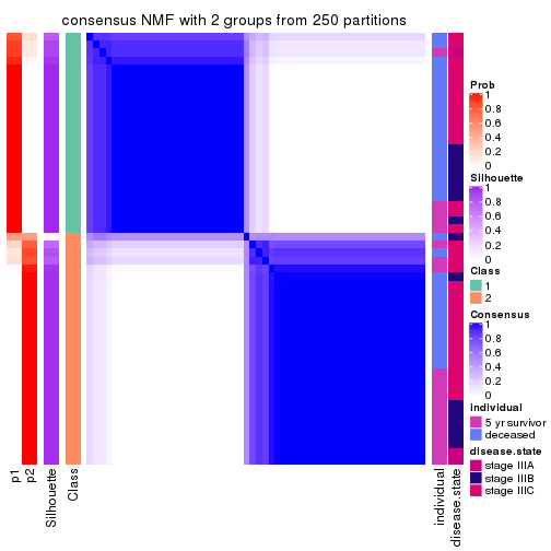
consensus_heatmap(res, k = 3)
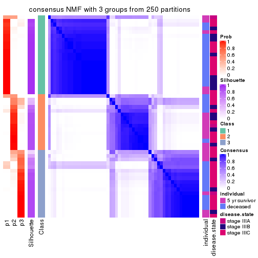
consensus_heatmap(res, k = 4)
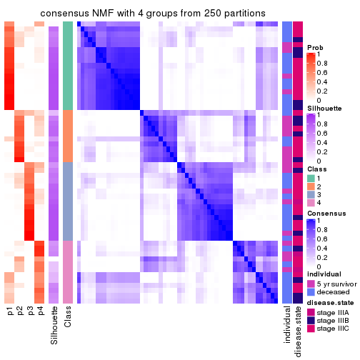
consensus_heatmap(res, k = 5)
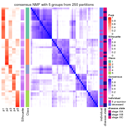
consensus_heatmap(res, k = 6)
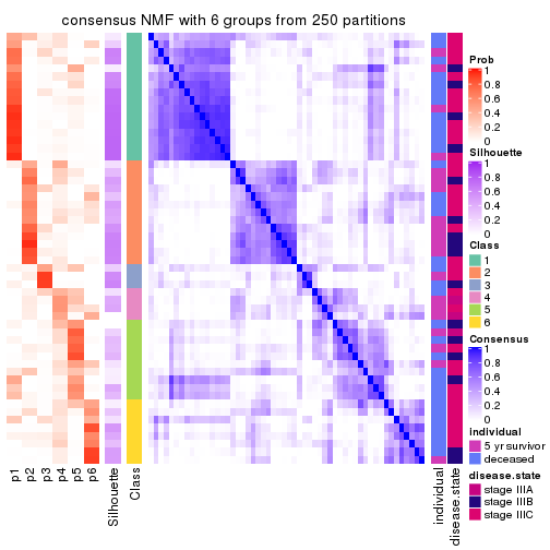
Heatmaps for the membership of samples in all partitions to see how consistent they are:
membership_heatmap(res, k = 2)
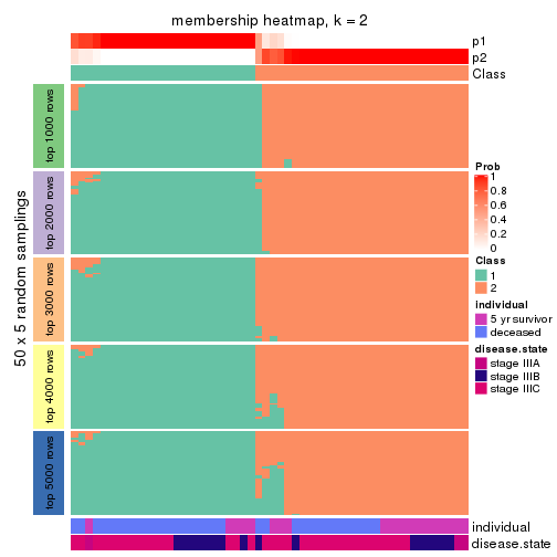
membership_heatmap(res, k = 3)
membership_heatmap(res, k = 4)
membership_heatmap(res, k = 5)
membership_heatmap(res, k = 6)
As soon as we have had the classes for columns, we can look for signatures which are significantly different between classes which can be candidate marks for certain classes. Following are the heatmaps for signatures.
Signature heatmaps where rows are scaled:
get_signatures(res, k = 2)
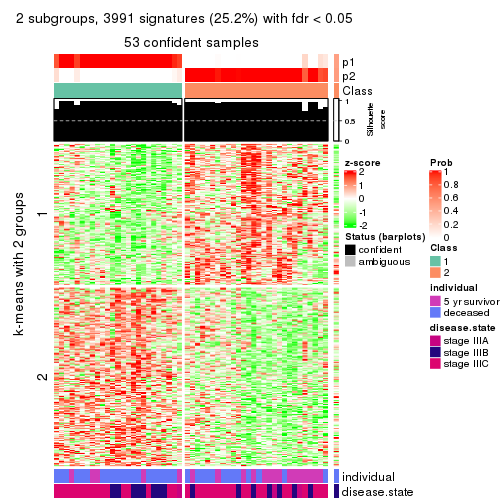
get_signatures(res, k = 3)
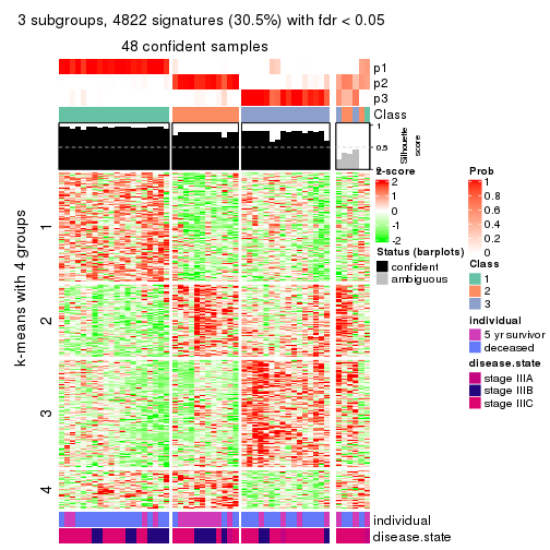
get_signatures(res, k = 4)
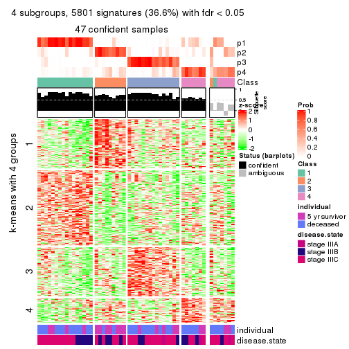
get_signatures(res, k = 5)
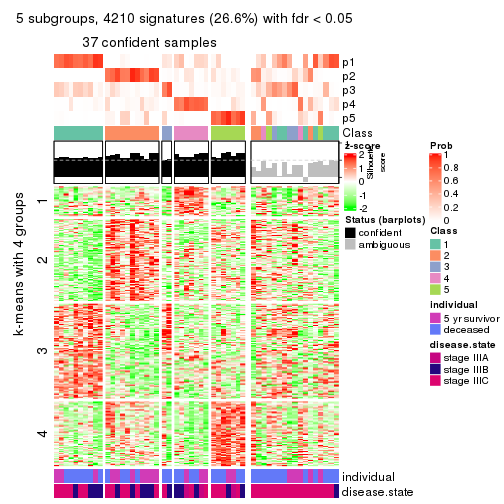
get_signatures(res, k = 6)
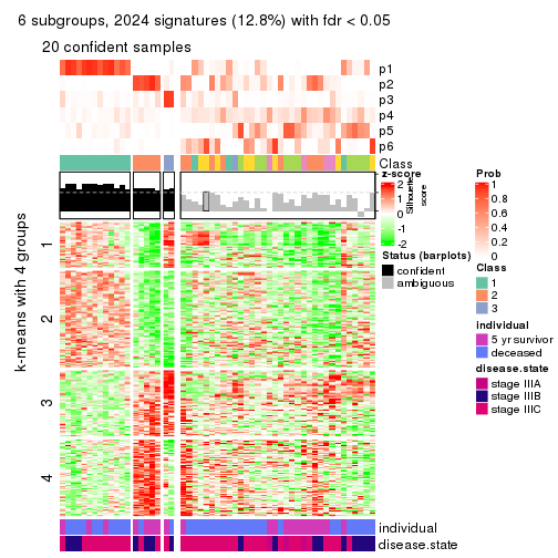
Signature heatmaps where rows are not scaled:
get_signatures(res, k = 2, scale_rows = FALSE)
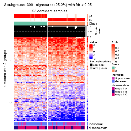
get_signatures(res, k = 3, scale_rows = FALSE)
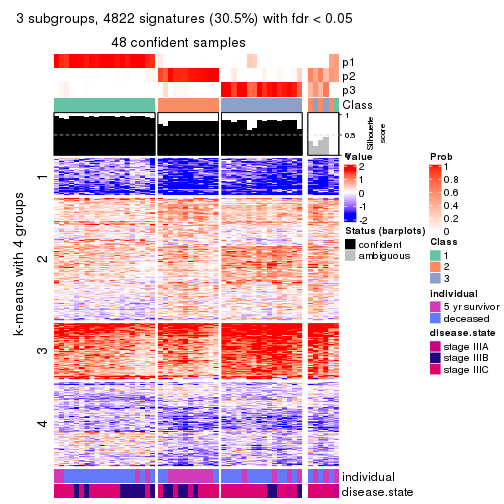
get_signatures(res, k = 4, scale_rows = FALSE)
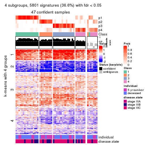
get_signatures(res, k = 5, scale_rows = FALSE)
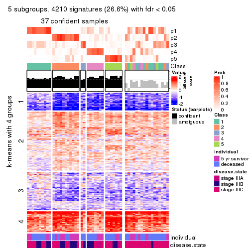
get_signatures(res, k = 6, scale_rows = FALSE)
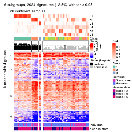
Compare the overlap of signatures from different k:
compare_signatures(res)
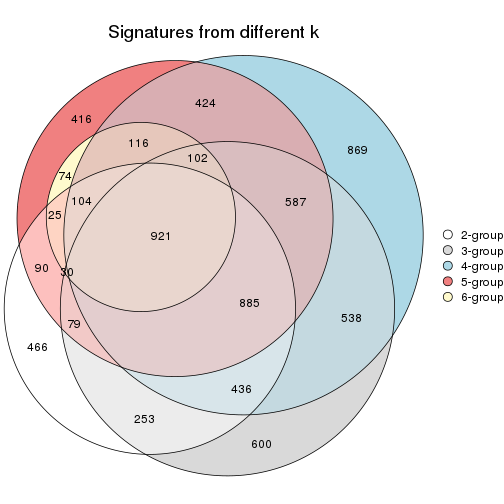
get_signature() returns a data frame invisibly. TO get the list of signatures, the function
call should be assigned to a variable explicitly. In following code, if plot argument is set
to FALSE, no heatmap is plotted while only the differential analysis is performed.
# code only for demonstration
tb = get_signature(res, k = ..., plot = FALSE)
An example of the output of tb is:
#> which_row fdr mean_1 mean_2 scaled_mean_1 scaled_mean_2 km
#> 1 38 0.042760348 8.373488 9.131774 -0.5533452 0.5164555 1
#> 2 40 0.018707592 7.106213 8.469186 -0.6173731 0.5762149 1
#> 3 55 0.019134737 10.221463 11.207825 -0.6159697 0.5749050 1
#> 4 59 0.006059896 5.921854 7.869574 -0.6899429 0.6439467 1
#> 5 60 0.018055526 8.928898 10.211722 -0.6204761 0.5791110 1
#> 6 98 0.009384629 15.714769 14.887706 0.6635654 -0.6193277 2
...
The columns in tb are:
which_row: row indices corresponding to the input matrix.fdr: FDR for the differential test. mean_x: The mean value in group x.scaled_mean_x: The mean value in group x after rows are scaled.km: Row groups if k-means clustering is applied to rows.UMAP plot which shows how samples are separated.
dimension_reduction(res, k = 2, method = "UMAP")
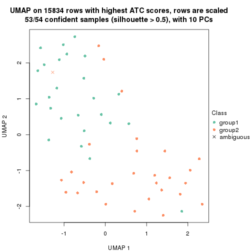
dimension_reduction(res, k = 3, method = "UMAP")
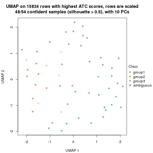
dimension_reduction(res, k = 4, method = "UMAP")
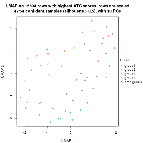
dimension_reduction(res, k = 5, method = "UMAP")
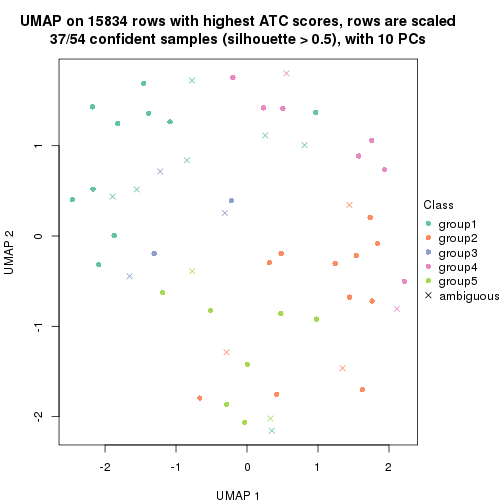
dimension_reduction(res, k = 6, method = "UMAP")
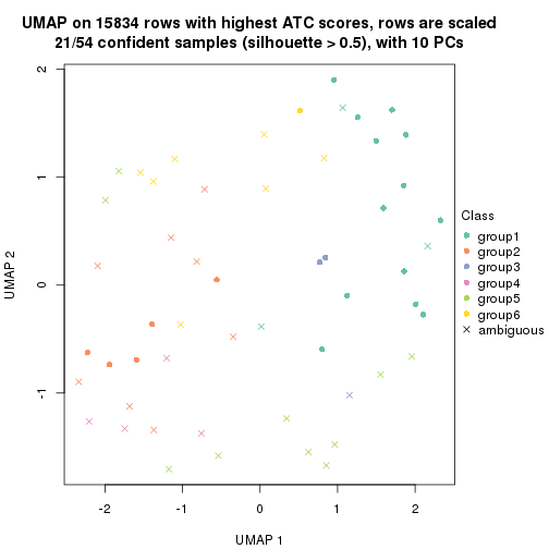
Following heatmap shows how subgroups are split when increasing k:
collect_classes(res)
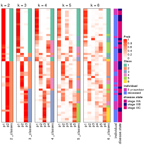
Test correlation between subgroups and known annotations. If the known annotation is numeric, one-way ANOVA test is applied, and if the known annotation is discrete, chi-squared contingency table test is applied.
test_to_known_factors(res)
#> n individual(p) disease.state(p) k
#> ATC:NMF 53 0.02554 0.783 2
#> ATC:NMF 48 0.00397 0.440 3
#> ATC:NMF 47 0.05578 0.525 4
#> ATC:NMF 37 0.32057 0.526 5
#> ATC:NMF 21 0.12704 0.397 6
If matrix rows can be associated to genes, consider to use functional_enrichment(res,
...) to perform function enrichment for the signature genes. See this vignette for more detailed explanations.
sessionInfo()
#> R version 3.6.0 (2019-04-26)
#> Platform: x86_64-pc-linux-gnu (64-bit)
#> Running under: CentOS Linux 7 (Core)
#>
#> Matrix products: default
#> BLAS: /usr/lib64/libblas.so.3.4.2
#> LAPACK: /usr/lib64/liblapack.so.3.4.2
#>
#> locale:
#> [1] LC_CTYPE=en_GB.UTF-8 LC_NUMERIC=C LC_TIME=en_GB.UTF-8
#> [4] LC_COLLATE=en_GB.UTF-8 LC_MONETARY=en_GB.UTF-8 LC_MESSAGES=en_GB.UTF-8
#> [7] LC_PAPER=en_GB.UTF-8 LC_NAME=C LC_ADDRESS=C
#> [10] LC_TELEPHONE=C LC_MEASUREMENT=en_GB.UTF-8 LC_IDENTIFICATION=C
#>
#> attached base packages:
#> [1] grid stats graphics grDevices utils datasets methods base
#>
#> other attached packages:
#> [1] genefilter_1.66.0 ComplexHeatmap_2.3.1 markdown_1.1 knitr_1.26
#> [5] GetoptLong_0.1.7 cola_1.3.2
#>
#> loaded via a namespace (and not attached):
#> [1] circlize_0.4.8 shape_1.4.4 xfun_0.11 slam_0.1-46
#> [5] lattice_0.20-38 splines_3.6.0 colorspace_1.4-1 vctrs_0.2.0
#> [9] stats4_3.6.0 blob_1.2.0 XML_3.98-1.20 survival_2.44-1.1
#> [13] rlang_0.4.2 pillar_1.4.2 DBI_1.0.0 BiocGenerics_0.30.0
#> [17] bit64_0.9-7 RColorBrewer_1.1-2 matrixStats_0.55.0 stringr_1.4.0
#> [21] GlobalOptions_0.1.1 evaluate_0.14 memoise_1.1.0 Biobase_2.44.0
#> [25] IRanges_2.18.3 parallel_3.6.0 AnnotationDbi_1.46.1 highr_0.8
#> [29] Rcpp_1.0.3 xtable_1.8-4 backports_1.1.5 S4Vectors_0.22.1
#> [33] annotate_1.62.0 skmeans_0.2-11 bit_1.1-14 microbenchmark_1.4-7
#> [37] brew_1.0-6 impute_1.58.0 rjson_0.2.20 png_0.1-7
#> [41] digest_0.6.23 stringi_1.4.3 polyclip_1.10-0 clue_0.3-57
#> [45] tools_3.6.0 bitops_1.0-6 magrittr_1.5 eulerr_6.0.0
#> [49] RCurl_1.95-4.12 RSQLite_2.1.4 tibble_2.1.3 cluster_2.1.0
#> [53] crayon_1.3.4 pkgconfig_2.0.3 zeallot_0.1.0 Matrix_1.2-17
#> [57] xml2_1.2.2 httr_1.4.1 R6_2.4.1 mclust_5.4.5
#> [61] compiler_3.6.0